Spot-On documentation
The official Spot-On documentation.
Spot-On allows you to analyze single particle tracking datasets. Spot-On fits a realistic kinetic model to the jump length distribution of the observed trajectories and provides estimates of the fraction bound (\(F\)) and diffusion coefficients (\(D\)) for either a two state (bound-free) or a three state (bound-free1-free2) model.
Spot-On is a libre/open-source software and exists both as a web-application and a command-line version.
This project owes a lot to Davide Mazza, who initially developed the conceptual framework implemented in Spot-On (see Mazza et al, 2012).
Browse the documentation for various versions of Spot-On:
The problem
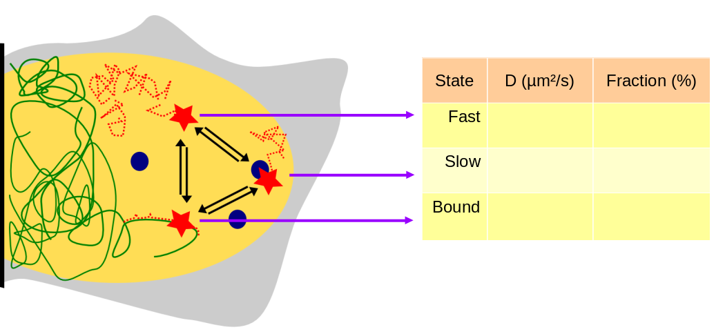
Within a cell, a DNA-binding factor diffuses and occasionally binds to DNA or forms complexes. Each of these states can be macroscopically characterized by an apparent diffusion coefficient and a fraction of the total population residing in this state. Thus, we are interested in extracting those parameters for each state. Note that even when the observed molecules are stably bound to DNA, they will still exhibit a nonzero diffusion coefficient (reflecting a mixture of the slow motion of chromatin (estimated to be around 0.01-0.02 µm²/s, Shinkai et al, 2016) --, the motion of the cell itself, microscope drift and possibly other factors).
To infer those parameters, single particle tracking (SPT) approaches can be implemented. In single particle tracking of nuclear proteins, cells are typically engineered to express a protein of interest either fused to a fluorescent protein or to a tag that can be conjugated to a synthetic dye (e.g. HaloTag). When the density of dyes in the focal plane is sufficiently low (because the number of expressed proteins is low, because the depth of field is extremely small or because only a fraction of the molecules are visible at a time), individual molecules appear as isolated spots that can be localized with a subpixel accuracy by fitting a 2D (usually Gaussian) function and performing tracking between successive frames. This yields a series of trajectories, each corresponding to the motion of a single protein-conjugated fluorophore.
Although extremely powerful, single particle tracking of nuclear factors is subject to several methodological difficulties detailed below:
Motion blur
When a diffusing particle is observed, it will keep diffusing while one frame is acquired. In this case, particles exhibit "motion blur", that is that the photons emitted by a fast-diffusing molecule appear spread across a higher surface than bound molecules. This has several consequences:
- First, fast-diffusing molecules show a reduced signal-to-noise ratio
- Second, these detections significantly deviate from the theoretical PSF (point-spread function) of bound molecules.
Because of these two effects, fast-diffusing particles are harder to detect, especially if PSF-fitting localization algorithms are used. Furthermore, because bound molecules are not affected by motion blur, molecules in the bound state tend to be overestimated because the fast-diffusing molecules are undercounted.
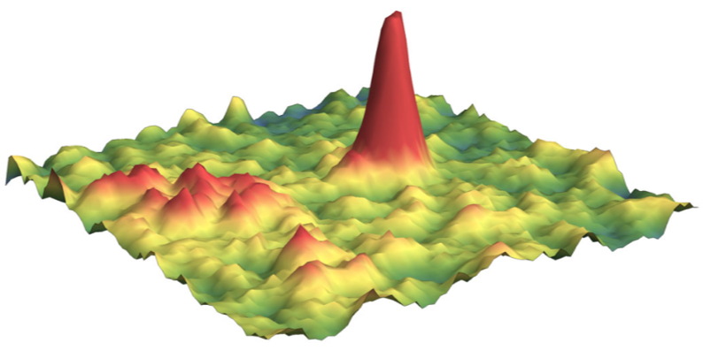
The picture below shows one frame containing two particles, one immobile particles appear as a very identifiable, Gaussian and symmetric spot (right red spot) whereas the fast-diffusing particle on the left is much harder to detect and very poorly resembles a point-emitter (spread out, left red spot).
Because motion blur results in under-detection of fast-diffusing particles, the amount of missed particles strongly depends on internal settings of the detection algorithm, and cannot readily be corrected after the acquisition. Section How to acquire a dataset details a few ways to circumvent these biases at the acquisition step.
In brief, the effect of motion blur can be mitigated by reducing the excitation pulse duration (to minimize the motion of the fast-diffusing population during one exposure) and the laser intensity (to keep the signal-to-noise sufficient).
Ambiguous tracking
As single particle tracking is intrinsically a low-throughput method, one may want to increase the density of tracked particles per frame in order to accelerate the data collection rate. However, as the density of particles increases, the tracking can become ambiguous. Furthermore, fast-moving particles are again more likely to be misconnected with other unrelated detections. This might result in a truncated jump length distribution, and thus a wrong estimation of the diffusion coefficient.
When imaging with a high density of particles, the nearest detection in the next frame might not be the same particle. In the limit of particles with high diffusion coefficients, it is likely that particles will "cross" each other and that one particle with be connected with another particle.
In practice, this leads to an under-detection of long jumps, because when a particle exhibits a long jump, the tracking algorithm is likely to pick another particle closer in space. This effect results in an underestimation of the fast-diffusing fraction and can be reduced by imaging at a low number of particles per frame. Section How to acquire a dataset details a few ways to circumvent those biases at the acquisition step.
Particles move out of focus
In addition to motion blur biases, that leads to fast-moving particle to be missed by the detection algorithm, particles diffuse out of the detection volume (usually a slice of ~ 1 µm thickness). This effect is virtually zero for bound molecule, but becomes significant for fast-moving particles, leading to an undercounting of this population. The animated graph below shows the jump length distribution of a molecule appearing in two states with respective diffusion coefficients \(D_1\) and \(D_2\) (expressed in µm²/s).
More precisely, the graph below displays the theoretical jump length distribution in case of an unlimited depth of field (solid line) and the simulation of the observed jump length distribution (dotted line) when particles are only observed within the depth of field of the objective (here set to 0.75 µm, see below for a method to measure it).
The cursors under the simulation allow tuning the diffusion coefficients of the two populations (\(D_1\) and \(D_2\)) and the proportion of the first population (\(p\)). From this graph, it appears (1) that as one increases the second diffusion coefficient (\(D_2\)), the discrepancy between the solid line and the dotted line increases, reflecting the fact that fast-diffusing particles tend to be under-counted in the observation through a setup with a finite depth of field.
In addition to \(D_1\), \(D_2\) and \(p\), this interactive graph allows you to play with the effect of the localization error \(\sigma\) and the exposure time \(\Delta t\). Note that this simulation does not take into account motion blur, so the undercounting of fast-diffusing particles is likely to be an underestimate.
Briefly, a reduced exposure time leads tends to limit the fraction of fast-diffusing particles moving out-of-focus from one frame to another. On the other hand, when the frame rate becomes too high, the detections are dominated by the localization error and inference become less and less accurate. Thus, a trade-off between the exposure time and the fast-diffusion coefficient has to be found.
| D1 (μm²/s) | |
| D2 (μm²/s) | |
| P | |
| σ (nm) | |
| Δt (ms) | |
| Show model with no depth of field correction |
|
From this representation, one can derive the fraction of particles that will move out of focus in the next frame as a function of the fast-diffusion coefficient and the exposure time (in this case, allowing one gap so that a particle out of focus for one frame can still be reconnected in the following frame).

This graph shows that fast-diffusing molecules (\(D> 5 \mu m/s\)) are extremely hard to track, even at a relatively high frame rate. For instance, when imaging at 100 Hz (10 ms per frame) a factor moving at 10 µm²/s (such as Halo-3xNLS), 40% of the particles move out of focus at each frame. This drastically limit the number of trajectories coming from the free population.
Furthermore, this graph only represents the fraction of particles remaining in focus after one frame. To get longer trajectories (more than two timepoints) is much harder, and is both limited by photobleaching and particles moving out of focus (detailed in section What limits the length of trajectories?.
Quickstart/tutorial
This section of the Spot-On documentation will guide you through a sample analysis with a couple of demonstration files and will provide you with an overview of Spot-On features and options.
Step 1: start an analysis with demonstration files
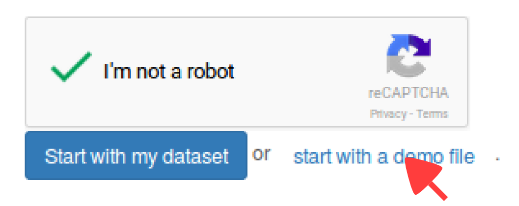
To access the demonstration files, go to the Spot-On homepage and scroll to the "Get Started section" (or alternatively click the Start spotting! button on the top menu. First fill in the "I'm not a robot" CAPTCHA. Then you have the option to either upload your own tracking files and start your analysis or start with demo files. We will use the demo files for the purpose of this tutorial.
This option will load the analysis page and will automatically import some demonstration file. Also, a custom and permanent URL is created. Your analyses will accessible from this URL until you choose to delete them. Do not share this URL if you want your datasets and analyses to remain private. You might want to bookmark it in order to reaccess the data later. Note that if you lose this address, there is no way for you to recover your files, since your upload is totally anonymous (we do not collect your identity or email address).
About the demonstration files
When you click on the "Start with a demo file" button, ten sample datasets are loaded. They are part of a bigger dataset described in details in the Datasets section that include single particle tracking of four nuclear proteins: histone H2B (H2B), Sox2, HaloTag-3xNLS and CTCF. These four proteins were imaged through a range of conditions, leading to approx. 1600 cells imaged in total.
By default, the ten imported files are five replicates of histone H2B (fused to both a HaloTag and a SNAP-tag in U2OS cells, labeled with the Halo-PA-JF646 dye and imaged at 74 Hz (that is 1000/74 = 13.5 ms per frame).
The five other files are five replicates of the transcription factor Sox2 (fused to a HaloTag in mouse embryonic stem cells and imaged in comparable conditions: labeled with PA-JF646 and imagied at 74Hz.
In this demo dataset, one of the goal is to get an idea of the dynamics of the Sox2 transcription factor. Indeed, an estimate of the fraction bound and diffusion coefficient of Sox2 provides a valuable insight into how this transcription factor regulates transcription. For instance, a low fraction bound and a high diffusion coefficient could suggest a highly dynamic regulation, but also a target search mechanism dominated by free diffusion. The H2B samples are provided as a reference for a protein that is known to be mostly bound to chromatin, in order to facilitate comparisons with more characterized systems.
Overview of the application
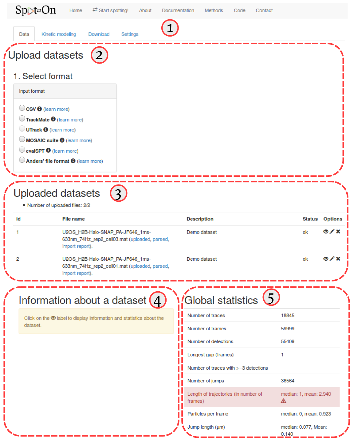
First of all, Spot-On is organized into four successive tabs. These tabs are populated one after the other (that is, for instance, the "Kinetic modeling" tab remains blank as long as no dataset has been uploaded in the "Data" tab, etc). The four tabs are (① in the screenshot below):
| Tab | Description |
|---|---|
| Data | This tab allows you to upload your datasets in various formats in a batch mode, to annotate them, and to see statistics both for individual datasets and for the ensemble of uploaded files. |
| Kinetic modeling | Performs the fit of the kinetic model according to specified parameters, display the jump length distribution and the corresponding fit. Allows to include or exclude files for analysis. Display and fits can be marked for download. |
| Download | This tab allows you to download the files marked for download in various formats (PDF, SVG, EPS, PNG, and ZIP archive). The ZIP archive contains the raw data, the fitting parameters and the fitted coefficients. |
| Settings | Allows you to erase the analysis (together with all the uploaded datasets). |
The "Upload dataset" region (② in the screenshot below), where you can upload from various file formats. Clicking on any of the format will display a box where you can enter additional upload parameters, and will ultimately display a drag-and-drop upload box. Accepted formats are described in more details in the Input formats section below.
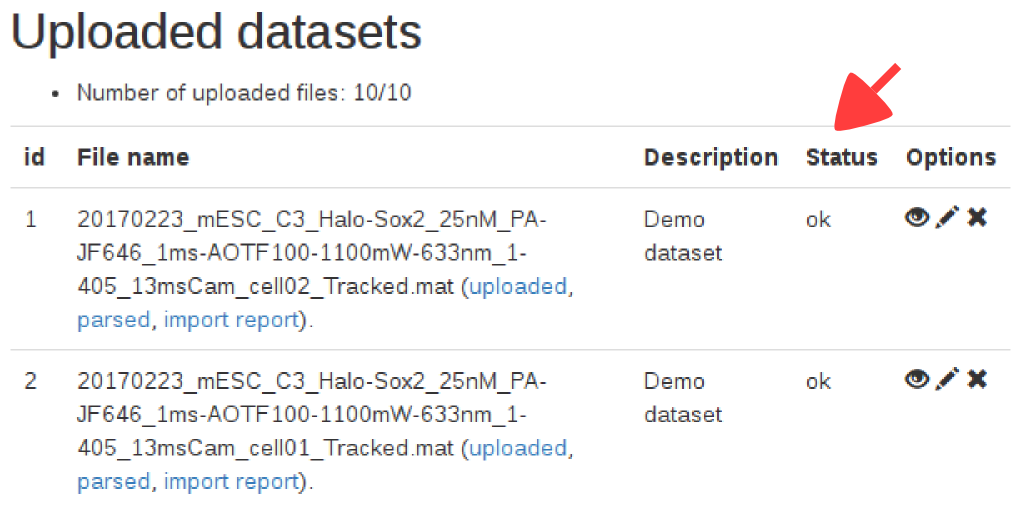
The "Uploaded datasets" region (③ in the screenshot below), that displays the uploaded datasets, together with their status (uploading, queued, error). The meaning of the descriptors in the "status" column in the upload box is detailed in the Status code of imported datasets section below. When clicking on the "eye" symbol () next to an uploaded dataset will display some statistics in the area ④. The meaning and details of the computation of each statistic is detailed in section Dataset statistics below. Finally, area ⑤ displays similar statistics as area ④, but for all the datasets pooled together.
Import
To proceed with the tutorial, several files have been loaded, they are named. They might get imported in a different order:
- mESC_C3_Halo-Sox2_PA-JF646_1ms-633nm_74Hz_rep2_cell01.mat
- mESC_C3_Halo-Sox2_PA-JF646_1ms-633nm_74Hz_rep2_cell02.mat
- mESC_C3_Halo-Sox2_PA-JF646_1ms-633nm_74Hz_rep2_cell03.mat
- mESC_C3_Halo-Sox2_PA-JF646_1ms-633nm_74Hz_rep2_cell04.mat
- mESC_C3_Halo-Sox2_PA-JF646_1ms-633nm_74Hz_rep2_cell05.mat
- U2OS_H2B-Halo-SNAP_PA-JF646_1ms-633nm_74Hz_rep2_cell01.mat
- U2OS_H2B-Halo-SNAP_PA-JF646_1ms-633nm_74Hz_rep2_cell02.mat
- U2OS_H2B-Halo-SNAP_PA-JF646_1ms-633nm_74Hz_rep2_cell03.mat
- U2OS_H2B-Halo-SNAP_PA-JF646_1ms-633nm_74Hz_rep2_cell04.mat
- U2OS_H2B-Halo-SNAP_PA-JF646_1ms-633nm_74Hz_rep2_cell05.mat
These files correspond to a subset of an experimental series spanning ~1500 cells in several conditions for various transcription factors and DNA-binding proteins, acquired at various framerates and durations of stroboscopic illumination. This dataset is described in more details in the Datasets section.
Five of these correspond to the transcription factor Sox2, which has been endogeneously tagged with a HaloTag and observed with the PA-JF646 organic dye (Grimm et al, 2016). The five other correspond to the Halo-tagged histone H2B imged under the same conditions.
Step 2: rename and tag the uploaded files
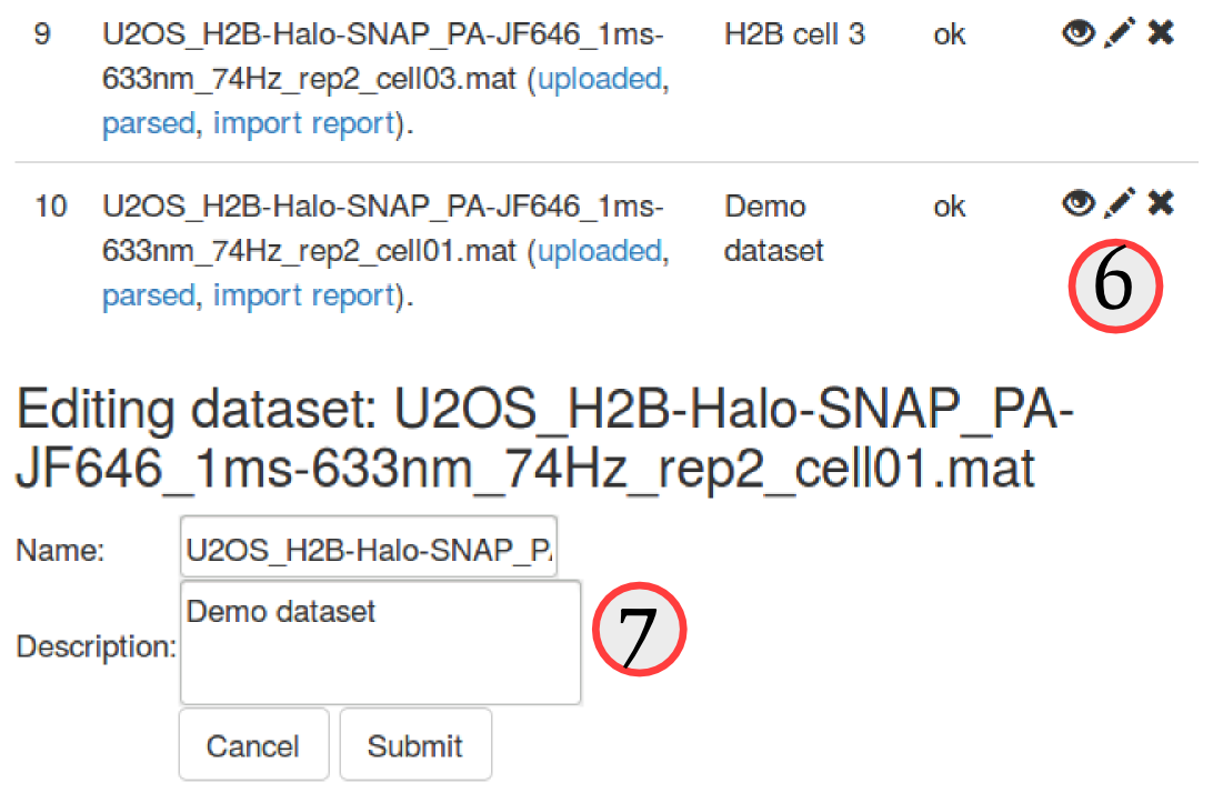
Since the naming convention of these files is a little bit cumbersome, let's first edit the description of each file to make it clearer. To do so, click on the "pencil" icon (, see ⑥) next to each uploaded dataset. An "edit" box will appear at the bottom of the "Uploaded datasets" area, and we can now either rename or add a more explicit description of the datasets. We choose to leave the name as is, but add a short description for each dataset, such as "H2B cell1", "H2B cell2", etc. (⑦)
Quality check
Now that we see a little bit clearer through the datasets, let's inspect a little bit the datasets, and try to assess the quality of the dataset. Spot-On provides a few quality metrics (statistics), accessible for each dataset by clicking the "eye" button ().
Step 3: Inspect a few quality metrics
Click on the "eye" button () next to the datasets and have a look at the metrics displayed. Make sure you familiarize yourself with those.
The table below summarizes the statistics computed for the first dataset (names mESC_C3_Halo-Sox2_PA-JF646_1ms-633nm_74Hz_rep2_cell01.mat.
| Statistic | Value |
|---|---|
| Number of traces | 6103 |
| Number of frames | 29997 |
| Number of detections | 15692 |
| Longest gap (frames) | 1 |
| Number of traces with >3 detections | 1813 |
| Number of jumps | 9589 |
| Length of trajectories (in number of frames) | median: 1, mean: 2.571 |
| Particles per frame | median: 0, mean: 0.523 |
| Jump length (µm) | median: 0.126, Mean: 0.236 |
Comment on the main features of the dataset. Although the number of jumps is not extremely high, we need to keep in mind that we plan to pool this dataset with four other datasets, which should overcome the limited size of this dataset. In case we encounter a dataset of unsuitable quality, we can exclude it by clicking the "cross" button () next to the dataset.
Once that we are confident about the quality of the uploaded data, we can proceed to the second tab, the "Kinetic modeling".
Kinetic modeling
Overview of the kinetic modeling tab
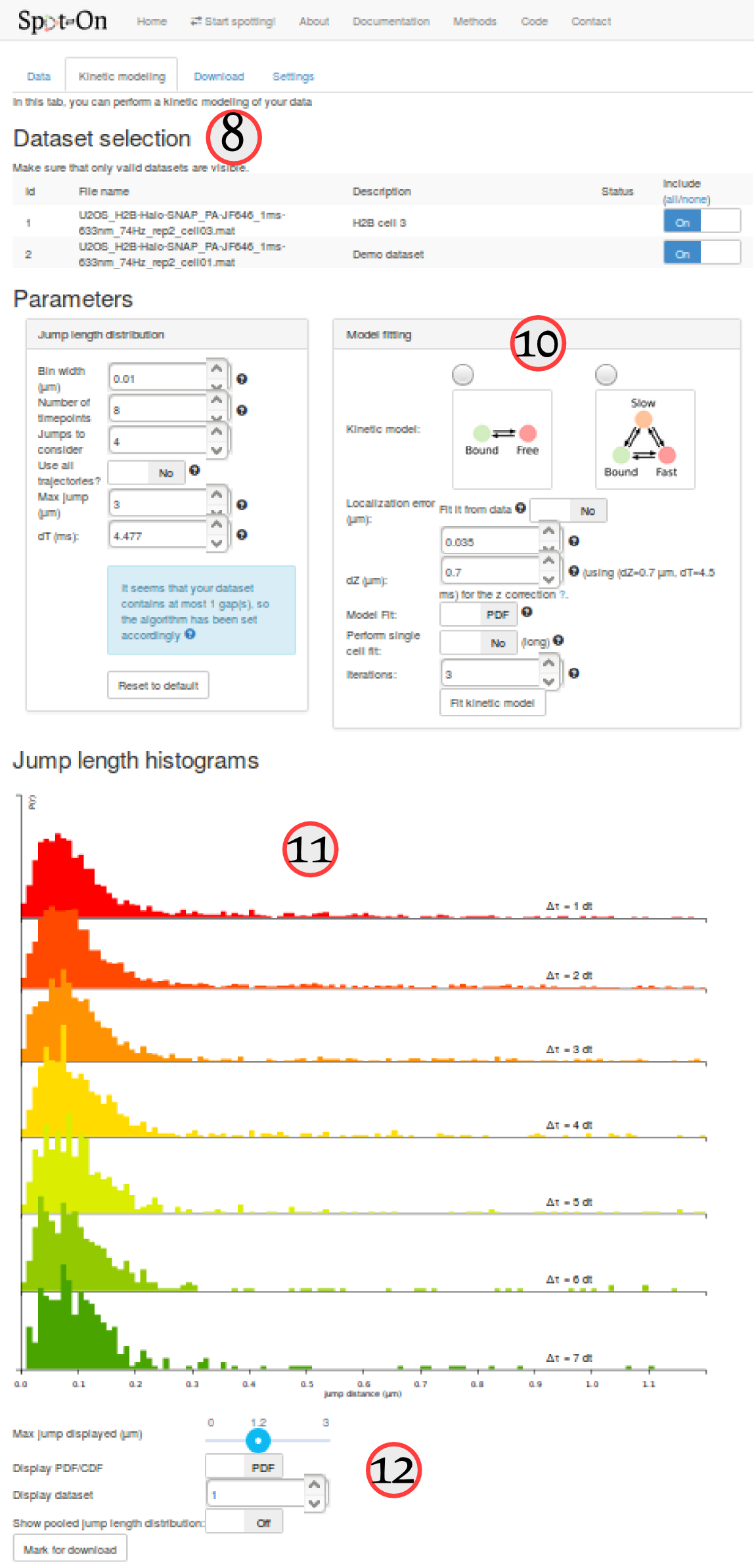
The "kinetic modeling" tab is divided in several sections:
| # | Section | Description |
|---|---|---|
| ⑧ | Dataset selection | This section lists all the uploaded datasets. For each fit of the model, you can choose whether to include one specific dataset for fitting or not. |
| ⑨ and ⑩ | Parameters | Parameters used to compute the empirical jump length distribution (⑨) and to fit it (⑨). This includes the choice of a 2-state vs. a 3-state model, the range of the tested parameters, etc. |
| ⑪ and ⑫ | Jump length histogram | This area contains the plot of the jump length distribution, overlaid with the fitted model (if evaluated). It also contains option to either visualize single datasets or the pool of the selected datasets. Finally, it contains an option to save an analysis for download. |
Computation of the jump length distribution
For the purpose of this tutorial, we'll simply fit the H2B and Sox2 datasets separately, and compare the two-state and three-state models based on their goodness of fit (assessed by the Bayesian Information Criterion, BIC).
Step 4: compute the empirical jump length distribution for the Sox2 datasets
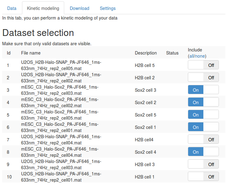
First, in the "Dataset selection" select the five Sox2 replicates. This is done by switching the "Include" toggle button to "On" next to the Sox2 datasets. Make sure that none of the H2B datasets are included.
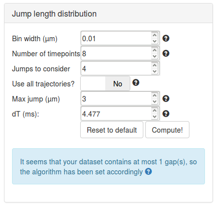
We can then set the parameters to compute the jump length distribution. We will mostly leave the parameters as default. Section Jump length distribution computation parameters describe the role of each parameter in more details.
Then click the Compute! button. After a few seconds, the jump length distribution is computed for all the datasets and appears under the "Jump length distribution" section.
The table below summarizes some key principles to properly set those parameters
| Parameter | Value | Default? | Comment |
|---|---|---|---|
| Bin Width (µm) | 0.01 | Y | The size of the bin used to build the empirical histogram of jump lengths. |
| Number of gaps allowed | 1 | Y | The number of gaps allowed by the tracking algorithm. This has to match the maximum number of gaps allowed by the tracking algorithm. |
| Number of timepoints | 8 | Y | The number of \(\Delta t\) to consider when fitting the model. Usually, higher values provide better results, provided that the histogram are sufficiently populated. |
| Jumps to consider | 4 | Y | The number of jumps per trajectory actually used to build the histogram. This is empirically useful to correct for overcounting of slow-molecules not accounted for by the corrections implemented in the algorithm (for instance for undercounting due to motion-blur). Here, for each trajectory, the first 4 jumps for each \(\Delta t\) (if possible) will be used to build the jump length histogram. For example, if Number of timepoints=8 and JumpsToConsider=4, a trajectory of 9 frames will contribute 4 jumps to 1dT, 4 jumps to 2 dT, …, and 2 jumps to 7 dT. This is a semi-empirical way of correcting for additional biases towards bound molecules. |
| Max jump (µm) | 3 | Y | The range of distances to build the histogram of jump lengths. This parameter has to be set so that the tail of the distribution is properly captured. Conversely, a value too high will disturb the fitting, that will be very sensitive to this potentially noisy tail. |
| dT (ms) | 13.5 | N | It is crucial to match this value with the acquisition rate of the dataset. Here 13.5 ms/frame. |
Step 5: play with the display options
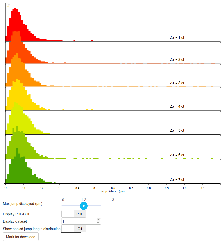
The graph displayed should be read as follows:
- Each row corresponds to a jump length distribution evaluated at a given \(\Delta t\). Since short trajectories are more frequent than long trajectories, higher \(\Delta t\) histograms tend to be less populated and appear less smooth (or more "noisy"). The number of rows is determined by the "Number of timepoints" parameter.
- The jump length distribution is computed for values ranging between 0 µm and 3 µm (this corresponds to the "Max Jump" parameter). However, by default, only the first 1.2 µm are initially plotted. To plot the full histogram (or alternatively, to zoom to the origin), the "Max Jump displayed" cursor, located under the plot can be adjusted.
- Then, by default, the jump length distribution is displayed for individual datasets. The displayed dataset is specified in the "Display dataset" box under the plot. It is often useful to take the time to review the jump length distribution of each single acquisition, in order to know which datasets might have to be excluded from further analysis.
- Once individual datasets have been reviewed, it is possible to display the pooled jump length distribution by clicking the "Show pooled jump length distribution" toggle button under the plot. This will compute the distribution for the selected datasets only (in our case, for all the Sox2 datasets). Pooled histograms appear with a hard, black boundary, and the included datasets are displayed under the graph. The updated graph might take a few seconds to render.
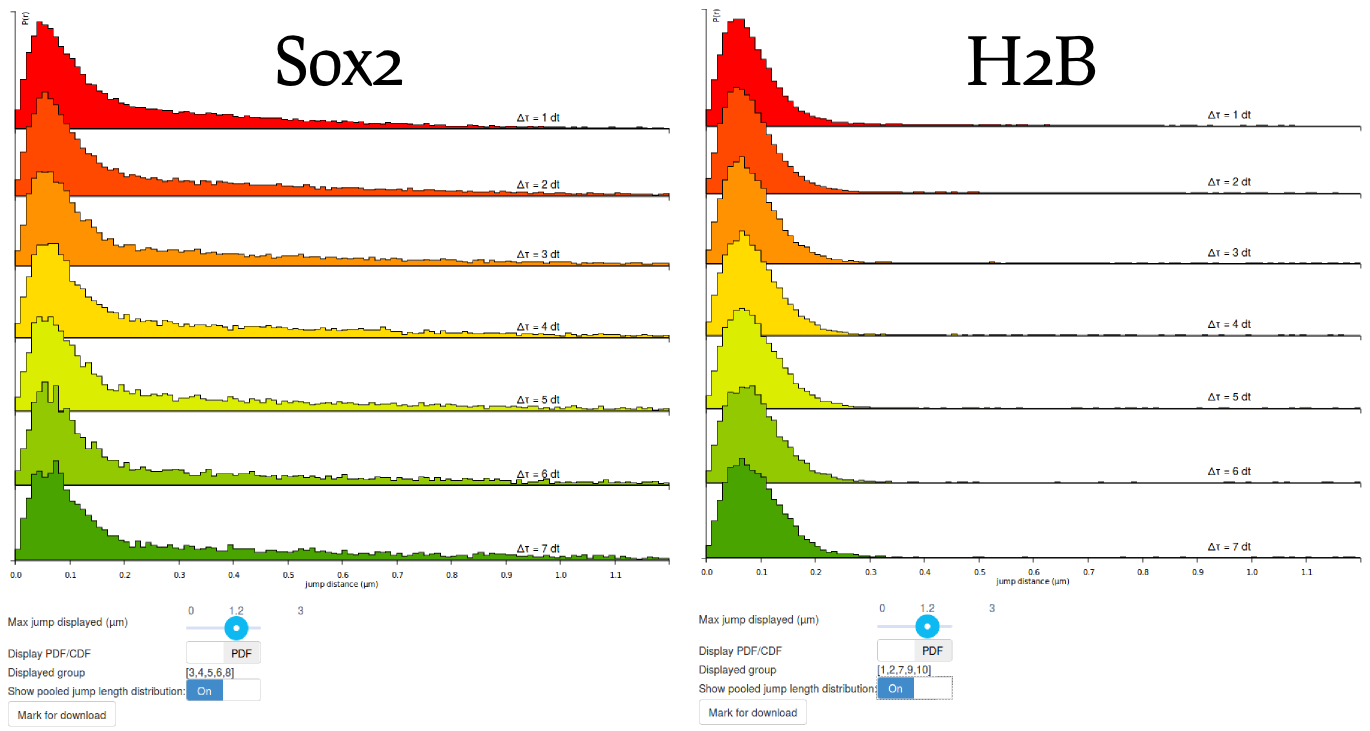
Step 6: compare the H2B and Sox2 jump length distributions
Before moving to the fitting, compare the pooled jump length distribution for Sox2 and H2B. To compute the H2B jump length distribution, simply uncheck the Sox2 datasets and select the H2B datasets in the "Dataset selection" area. Then click the Compute! button in the "Jump length distribution parameters" box. The two histograms are displayed below. What can you tell from that? Does it match your knowledge of H2B and Sox2?
When looking at the two histograms side-by-side, the two look very similar at short time scales (up to 200 nm), suggesting that the two proteins show a bound fraction. The dispersion around ~70 nm is likely to be characteristic of a combination of localization error (similar at all time scales, from \(1\Delta t\) to \(7\Delta t\) and of slow diffusion of chromatin (that slowly spreads when looking at higher \(\Delta t\).
Then, when considering higher distances, the histograms differ significantly, with Sox2 exhibiting a "heavy tail" whereas H2B lacks it. This reflects the fact that H2B is mostly bound whereas Sox2 has a significant freely-diffusing fraction. The modeling approach presented in the next steps of the tutorial will allow us to better characterize this diffusing state.
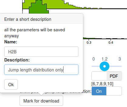
Step 7: mark one jump length distribution for download
Before moving to the fitting of the data, let's save this last plot. We will download it later (from the "Download" tab). To do so, click the Mark for download button at the bottom of the page. This will prompt a small form where you can enter a name and a description that will be used as a reminder when you download the file. Also, display again the jump length distribution for Sox2 (by selecting the appropriate files and clicking the and Compute! button in the "Jump length distribution parameters" box) and save Mark it for download too. We'd get back to these saved analyses later.
Model fitting
Now that we are familiar with the computation and display of the jump length distribution, let's now move to model fitting!
Spot-On fits the jump length distribution, as defined by the parameters of the "Jump length distribution" box. The fitting parameters are defined in the "Model fitting" box.
Step 8: fit a two-state model to the H2B data
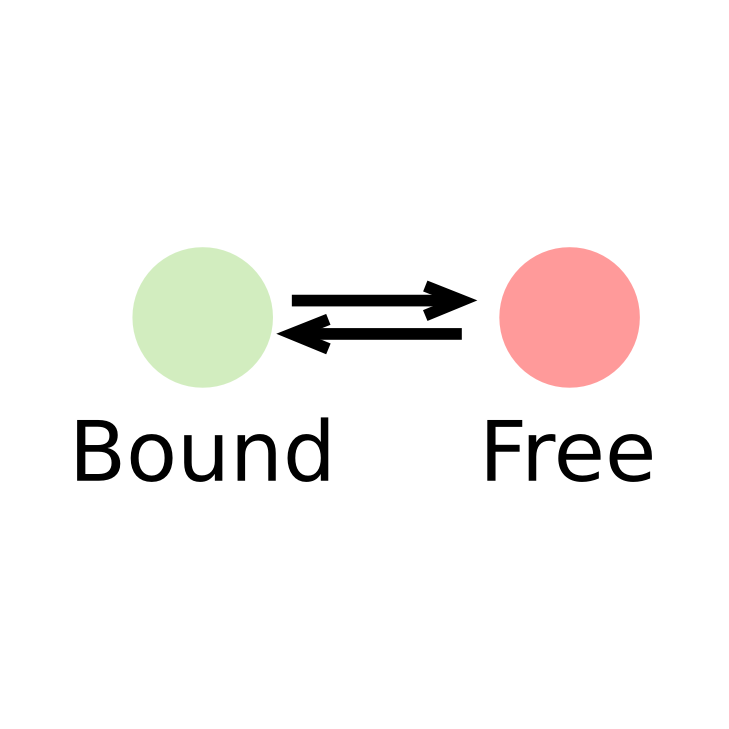
Let's first try to fit a two-state model. Click on the picture of the two-state kinetic model (Bound-Free). Specific parameter for this model unfold. Let's take a minute to quickly review them (a more detailed description of each parameter is presented in Section Fitting parameters, a short description is shown below).
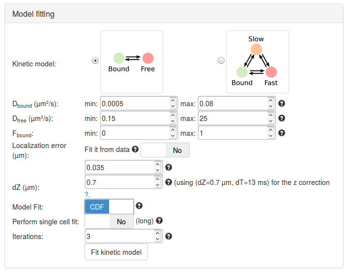
Having now reviewed the parameters, we can click the Fit kinetic model button. A "spinning wheel" will appear next to the button while the fit is being performed and will get displayed when the fit completes.
| Parameter | Value | Default? | Description/Comments |
|---|---|---|---|
| Kinetic model | 2-state model | N | |
| Dbound (µm²/s) | [0.005, 0.8] | Y | The range of diffusion coefficients for the bound fraction. It is based on a wide plausible range of chromatin diffusion coefficients. |
| Dfree (µm²/s) | [0.15, 25] | Y | The range of diffusion coefficients for the free fraction. These numbers encompass a wide range of free-diffusion coefficients. Note that for diffusion coefficients > 10 µm²/s, motion blurring can become a very important issue. |
| Fbound | [0,1] | Y | The range for the fraction bound. |
| Localization error (µm) | 0.035 | Y | See How to measure the localization error? below. |
| dZ (µm) | 0.7 | Y | The estimated detection range in z. |
| Model Fit | CDF | N | Select whether the model will fit the jump length distribution (that is the probability density function, PDF), or the cumulative jump length distribution (CDF). |
| Perform single cell fit | No | Y | If "Yes", each individual dataset will be fit. Since our uploaded files are replicates of the same experiment, we want to pool them together. |
| Iterations | 3 | Y | The number of times the solver will independently be initialized. |
When adjusting the dZ parameter (in the fitting parameters box), you will notice that the mention next to the dZ box changes. The displayed values relate to precomputed coefficients required to perform the correction for particles moving out of focus (see the Methods section). These parameters are termed \((a,b)\) and were precomputed over a grid of depths of field (dZ) and exposure times (dT).
However, even though we tried to be as comprehensive as possible in our simulations to derive \((a,b)\), the condition that matches exactly the acquisition settings might be missing. The displayed parameters represent the closest match of the acquisition parameters (dT, dZ) in our simulated database. For most acquisitions setup, the closest precomputed value lies within 0.5 ms and 100 nm of the empirical value.
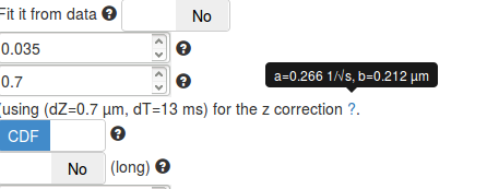
It is important to make sure that the set of displayed parameters is not too far from the real acquisition settings, else, the computed z correction might be biased.
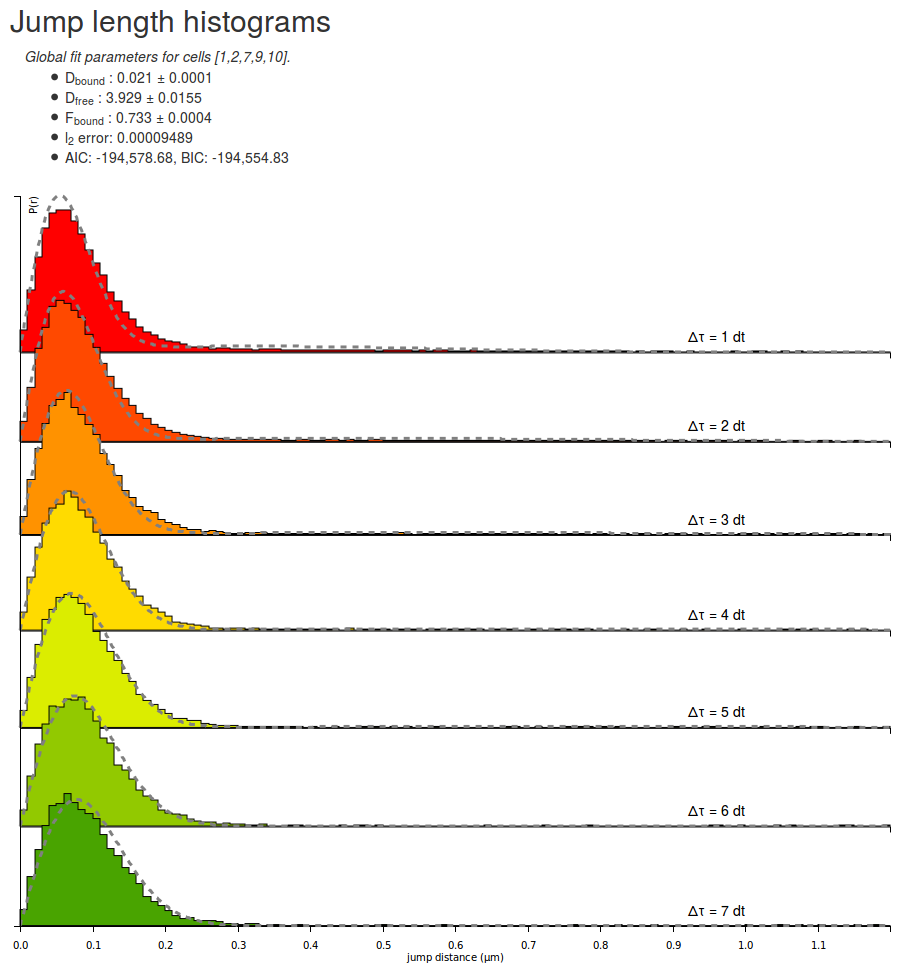
Let's take some time to quickly look at the parameters returned by the fitting routine for the H2B datasets. Note that due to different initialization values, the returned parameter can differ from execution to execution:
| Parameter | Value |
|---|---|
| Dbound | 0.021 µm²/s |
| Dfree | 3.929 µm²/s |
| Fbound | 0.733 |
| l2 error | 0.00009489 |
| AIC | -194578 |
| BIC | -194554 |
A few comments arise. First, the estimated fraction bound is about 70 %, which is expected from a strongly DNA-associated protein such as H2B. The associated coefficient with the bound population is close to zero (0.021 µm²/s) whereas the diffusion coefficient for the free population (3.93 µm²/s) matches previous knowledge of the dynamics of the protein.
Furthermore, the \(\ell_2\) error (the mean square error) is \(\lt 10^{-4}\), which can be considered as acceptable (note that this value is not a hard limit and depends on several parameters, including the bin width and the max jump parameters), even though significant misfit appear at low and high \(\Delta t\): at \(1\Delta t\), the fitted distribution is fading faster than the empirical one, whereas at \(7\Delta t\), the opposite effect happens. This might be a sign that the protein of interest exhibits anomalous diffusion, or more generally that the model does not fully explain the dynamics of the molecule.
Finally, the AIC (Akaike Information Criterion) and BIC (Bayesian Information Criterion) criteria are provided to allow model comparison. These are two criteria that can be used to compare models and to get hints about which model fits the data best while penalizing for the number of parameters, in order to avoid overfitting.
More specifically, the 3-state model provided by Spot-On has more free parameters than the two-state model (two extra parameters: the "slow" diffusion coefficient and the fraction of the slow-moving fraction). This additional degrees of freedom almost always a better fit than the 2-state model. The AIC and BIC criteria take this difference in the number of parameters and establish a trade-off between the quality of fit (that increases with the number of model parameters) and the number of parameters, in our case penalizing the possible overfitting of the 3-state model.
Although these criteria are useful when comparing the fit of one dataset compared to various models, they cannot be used to assess the quality of fit per se.
Step 9: mark the plot for download
Then, we can save the displayed fit by clicking the Mark for download button.
Step 10: fit the Sox2 dataset with a two-state model
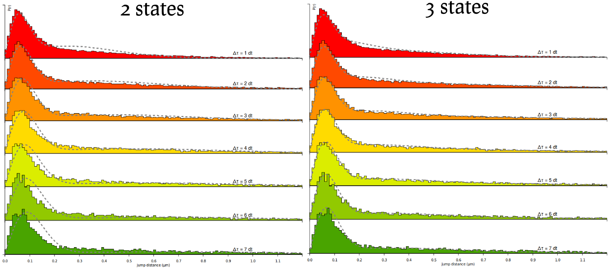
We can now proceed similarly to derive the fit for the Sox2 datasets. The resulting fit is shown below, next to a fit using a three-state model. Notice in this plot that significant misfit occurs: at high \[\Delta t\) the model estimates predicts that the bound fraction should have bigger displacements than what actually is. This characterizes a model mismatch and suggest the use of a three-state model.
Step 11: fit a three-state model
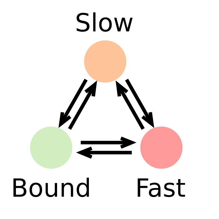
Finally, we can now see how the quality of the fit increases by running the fit again, but with a 3-state model. Select the 3-state model icon (Slow-Bound-Fast) on the "Model fitting" box. New parameters appear, very similarly as with the two-state model. We will leave the parameters to their default values, except for the CDF fit. Then click the Fit kinetic model button and wait a until the fitting completes. Observe how the quality of fit evolves, and the parameters and estimated fractions.
| Parameter | Value |
|---|---|
| Dbound | 0.030 µm²/s |
| Dfree | 2.410 µm²/s |
| Fbound | 0.340 |
| l2 error | 0.00039589 |
| AIC | -164571 |
| BIC | -164547 |
| Parameter | Value |
|---|---|
| Dbound | 0.012 µm²/s |
| Dslow | 0.595 µm²/s |
| Dfast | 4.016 µm²/s |
| Fbound | 0.256 |
| Fslow | 0.258 |
| l2 error | 0.00014930 |
| AIC | -185061 |
| BIC | -185021 |
Based on the information criteria, it is clear that the 3-state model provides a better fit to the data, even when penalizing for the number of parameters.
Step 12: compare the two-state fits of H2B and Sox2 datasets
Let's then fit the H2B data with a two-state model, as described in Step 10 for Sox2 (make sure that you select the right datasets before clicking the Fit button). Once the fit has completed, compare the fitted coefficients between the two proteins:
| Parameter | Value |
|---|---|
| Dbound | 0.030 µm²/s |
| Dfree | 2.410 µm²/s |
| Fbound | 0.340 |
| Parameter | Value |
|---|---|
| Dbound | 0.023 µm²/s |
| Dfree | 3.84 µm²/s |
| Fbound | 0.70 |
Notice that the bound diffusion coefficient are very similar, likely reflecting the diffusion coefficient of DNA/chromatin itself, while the free diffusion coefficients are different, and are likely to reflect different exploration modes of the two proteins. Also notice that the fraction bound are widely different: whereas H2B is mostly bound (70%), Sox2 appears mostly free.
Download
Step 13: download the marked analyses
Finally move to the "Download" tab, where all the analyses we marked for download are stored. The view should look as below:
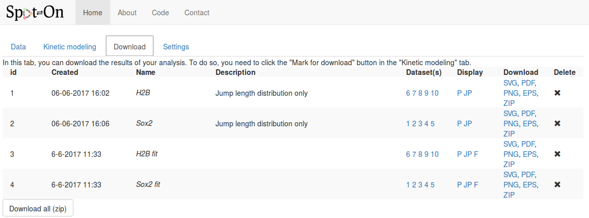
For each analysis marked for download, the following fields are displayed, in addition to the time of the analysis and the name and description we provided in the previous tab:
| Column | Description |
|---|---|
| Name & description | The name & description we provided in the previous tab. |
| Datasets | The list of datasets included for this plot. Hovering over the numbers displays the full name and description of the dataset. |
| Display | Descriptor corresponding to the type of plot displayed. Hover over the descriptor to see a short description:
P: display of the probability density function,
JP: display the pooled jump length distribution,
F: pooled fit displayed |
| Download | Download the corresponding analysis in various formats. The ZIP archive contains all the formats, the raw data, the display parameters and the fitted coefficients (if any). |
| Delete | To delete this analysis. |
Software reference
This section describes in detail the function of all the features and options implemented into Spot-On.
Input formats
Spot-On accepts tracking files from the following software and raw CSV (column naming below): TrackMate, MOSAIC suite, evalSPT (a variant of MTT) and an additional custom Matlab format. Sometimes, the importer can be a little bit picky. We provide sample files for these formats so that you can potentially study them. In case you have a problematic file, do not hesitate to contact us and email us the problematic file.
CSV (Comma-separated values)
Files can be uploaded as raw CSV files. Make sure that the separator indeed is a comma (,). Importing from a tab-separated or semicolon-separated file will not work. The CSV file should have a header line and contain the following columns. Any other column will be ignored. The order of the columns does not matter. Note that the header naming convention is case sensitive. This importer assumes that tracking has been performed already and that sets of detections were assigned a numerical index (or trajectory id).
| frame | t | trajectory | x | y | |
|---|---|---|---|---|---|
| Format | (integer) | (float) | (integer) | (float) | (float) |
| Description | Frame number | Time (in s) | The trajectory id | x position of the particle (in µm) | y position of the particle (in µm) |
TrackMate
TrackMate is an ImageJ/Fiji plugin that can perform various types of tracking and export the traces to various file formats. Spot-On can import from its XML and CSV export.
Note that the file has to be exported from the last panel of the wizard (clicking the "Save" button at the bottom of the window will produce a XML file that cannot be read by Spot-On). A screenshot of TrackMate's export interface is displayed below.
TrackMate saves the framerate of the movie in the exported XML file. However, for some reasons, this can be unproperly set. See the ImageJ documentation about how to set up the framerate. The framerate has to be set in 'ms' (milliseconds) to be recognized by Spot-On.
In the .xml file exported by TrackMate, the recorded framerate is indicated in the frameInterval field, and the saved unit in the timeUnits field. You can safely manually edit those values in case they were not saved when performing the tracking.
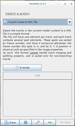
Again, the export can be performed by selecting either "Export tracks to a XML file" or "Export tracks to a CSV file". Clicking on "Save" will not work.
Download sample file (CSV) Download sample file (XML)UTrack
u-track is an Matlab software that can perform various types of tracking and export the traces to a custom Matlab format. Spot-On can import it provided that no branching was allowed in the settings. Below are some suggested parameters:
gapCloseParam.timeWindow = 1; %maximum allowed time gap (in frames) between a track segment end and a track segment start that allows linking them.
gapCloseParam.mergeSplit = 0; %1 if merging and splitting are to be considered, 2 if only merging is to be considered, 3 if only splitting is to be considered, 0 if no merging or splitting are to be considered.
gapCloseParam.minTrackLen = 1; %minimum length of track segments from linking to be used in gap closing.
Note that if gapCloseParam.mergeSplit is set to 1, Spot-On will not be able to read the format and will silently fail.
We are very grateful to Khuloud Jaqaman (UT Southwestern) and Gaudenz Danuser (UT Southwestern) for precisions about this file format.
Download sample file (mat)MOSAIC suite
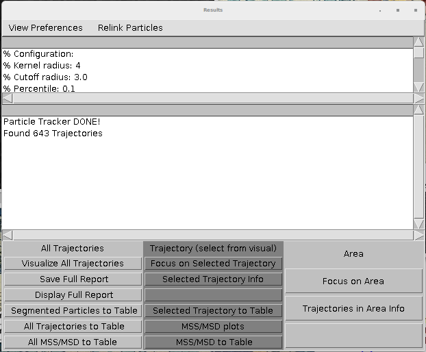
MOSAIC suite is an ImageJ/Fiji plugin that can perform tracking and export the traces as an ImageJ table. This table can be further exported to CSV. The table is displayed by clicking the "All Trajectories to table" and "Selected Trajectories to table" at the end of the wizard.
evalSPT
evalSPT (software mentioned in Normanno et al, 2015) produces a TSV format (tab-separated values), with no header, with the first columns ordered as follows. Additional columns might be present but will be ignored. An example file is provided below.
| Column 1 | Column 2 | Column 3 | Column 4 | Column 5 and more |
|---|---|---|---|---|
x position of the particle (in pixel) |
x position of the particle (in pixel) |
frame number | trajectory number | These columns are ignored |
Matlab file format
Spot-On also accepts a custom Matlab file format. An example is provided below. The trackedPar variable is a structured array. Each element of this array corresponds to one trajectory. Each trajectory contains several fields: xy, t, frame. Each of these fields is a 2D-matrix with 2, 1 and 1 columns, respectively and a number of rows corresponding to the number of detections for this trajectory.
Note that this format (in particularx the shape of the objects) has to be followed rigorously for Spot-On to be able to import it. In particular, a \(N\times 1\) matrix is different from a \(1\times N\) matrix.
Download sample fileDescriptors of imported datasets
When a dataset is uploaded, a column "status" is displayed, showing the state of the import. Below is the meaning of the status codes displayed:| Status code | Meaning |
|---|---|
| Uploading | The dataset is being transferred to the server. |
| Queued | The dataset has been uploaded, and will be checked for import. |
| Ok | The dataset was successfully imported. |
| Error | Something went wrong with the import process, and the file could not be imported. The file has been deleted from our servers and you might want to check the file format and upload it again. |
Note that once the dataset is marked as "ok", the jump length distribution might still be computing in the background. The content of the second tab only appears when this computation is done, which might take a few seconds.
Dataset statistics
Once a dataset has been successfully imported, several statistics are displayed and allow you to get a quick overview of the data, and spot dubious datasets or datasets that might likely need to unreliable analyses. We detail below how theses statistics are computed and what are suggested reference values.
| Statistic | Meaning | Why it matters? |
|---|---|---|
| Number of traces | The number of trajectories in the dataset. Trajectories can be singletons (one detection) and arbitrary long. | A low number of traces will cause the jump length histograms to be noisy and limit the accuracy of model-fitting |
| Number of frames | The duration of the acquisition (in frames). This is inferred as the maximum index of the "frame" field. If you do not have detections at the end of the movie, this number can be lower than the true number of frames. | This number should more or less match the number of frames for the acquisition of this dataset. |
| Number of detections | The number of particles detected. | Too low a number of detections is problematic since background noise will make a bigger contribution, whereas too high may suggest tracking errors. |
| Longest gap (frames) | The maximum number of frames during which a particle disappeared before being tracked again by the tracking software. | A number of gaps >2 frames is very likely to yield significant tracking errors. |
| Number of traces with ≥ 3 detections | Number of trajectories that contain three detections or more | This indicates whether histograms can be populated for \(\Delta t > 1\). |
| Number of jumps | The number of tracked translocations (only \(1\Delta t\) translocations are reported) | Jumps are used to build the histogram of jump lengths, so this is probably one of the most relevant metrics to evaluate the quality of the dataset. |
| Length of trajectories (in number of frames) | Provides the mean and median length of trajectories. | Useful also for assessing dataset quality. |
| Particles per frame | The mean and median number particles per frame. | A median number higher than one indicates the risk of tracking errors. |
| Jump length (µm) | The mean and median translocation distance | In general, the mean translocation should be significantly bigger than the localization error. |
Jump length distribution computation parameters
The empirical jump length distribution is computed according to several parameters that are detailed below.| Parameter | Meaning |
|---|---|
| Bin width (µm) | how finely to do binning for PDF fitting and plotting in units of micrometers. Generally, 0.010 μm or 10 nm is reasonable, but if you have very small amounts of data you may want to increase it. |
| Number of timepoints | How many time points to consider. If you allow \(N\) time points, this corresponds to considering displacements with a maximal time-delay of \((N-1)\Delta t\). Generally, we do not recommend going much above 50-60 ms unless you have an a very large number of trajectories and/or very long trajectories, since otherwise, the displacement histograms at longer \(\Delta t\) tend to be undersampled. |
| Jumps to consider | The number of jumps per trajectory actually used to build the histogram. This is emppirically useful to correct for overcounting of slow-molecules not accounted for by the corrections implemented in the algorithme (for instance for undercounting due to motion-blur). Here, for each trajectory, 4 jumps (if possible) will be used to build the jump length histogram. For example, if Number of timepoints=8 and JumpsToConsider=4, a trajectory of 9 frames will contribute 4 jumps to 1dT, 4 jumps to 2 dT, …, and 2 jumps to 7 dT. This is a semi-empirical way of correcting for additional biases towards bound molecules. This parameter is ignored if "Use all trajectories" is set to Yes. |
| Use all trajectories? | If "Use all trajectories" is set to "Yes", the previous parameter ("Jumps to consider" is being ignored. If set to "Yes", all displacements will be used from each trajectory. If set to "No", then the number of displacements is determined by the "Jumps to consider" variable. A trajectory of \(N\) frames, will contribute \(N-1\) displacements to the \(1\Delta t\) histogram, \(N-2\) displacements to the \(2\Delta t\), histogram, ..., \(N-k\) displacements to the \(k\Delta t\) histogram. |
| Max jump (µm) | this parameter affects data-processing. For binning displacements, a maximum displacement has to be set, so this parameter should be set to a large value that should be at least as big as the largest displacement. Generally, 5.05 μm is reasonable for single-molecule tracking data in mammalian cells. |
| dT (ms) | Time delay between frames in units of milliseconds. |
Fitting parameters
| Parameter | Meaning | Why it matters? |
|---|---|---|
| Kinetic model | The number of diffusive states in the model. Spot-On supports 2- or 3-state. In most single-molecule tracking experiments of molecules that can engage scaffolds (e.g. transcription factors, which may bind chromatin), one of these states will correspond to a bound state. In the case of Halo-CTCF in human U2OS cells, this will manifest itself as the chromatin-bound state of CTCF exhibiting a very small \(D\) for the bound state which likely corresponds to slow diffusion of chromatin. The other states will correspond to freely diffusive states. | |
| Dfree, Dbound, Dslow, Dfast | Allowed lower and upper bound for the faster diffusion constant for the model-fitting in units of μm²/s for the free (2-state model), bound (all models), slow (3-state model) or fast (3-state model), respectively. | |
| Fbound, Ffast | The range of possible values for the bound fraction (all models) and the fast-diffusing fraction (3-state model), respectively. | |
| Localization error (µm) | If "Fit from data" is set to "No", you can provide the localization error with which single-molecules were localized. If "Fit from data" is set to "Yes", Spot-On will try to infer this from the model-fitting. In that latter case, you need to provide an exploration range for these values. In the datasets provided with Spot-On, the localization error was around 35 nm. If the localization error parameter is set inaccurately, this will generally show up through poor fitting of the bound state and will cause the estimation of the bound diffusion constant to be inaccurate. | |
| dZ (µm) | Axial observation slice in units of micrometers. This parameter will depend somewhat on signal-to-noise conditions and imaging modality. But for a typical setup (HiLo or epi illumination, HaloTag or SNAP-Tag dyes), this is likely to be around 0.7 μm. The parameters tell Spot-On how far out-of-focus a molecule can be before it fails to be detected and it is important for accurately correcting for diffusing molecules gradually moving out-of-focus and thus being undersampled at longer time-intervals. In most cases 0.7 μm is reasonable, but for details on how to measure this please see (Hansen et al. (2017). | |
| Perform single cell fit | When set to "Yes", each single uploaded file will be analyzed and fitted separately. This is useful for assessing how much cell-to-cell variability there is and for determining whether a single outlier is biasing the results, but also very slow, since fitting merged data takes about the same amount of time as fitting a single cell. | |
| Model Fit | Determines whether fitting will be performed to the displacement histograms (PDF) or to the cumulative distribution function of displacements (CDF). We have performed Monte Carlo simulations and CDF-fitting is always more precise, whereas PDF-fitting tends to slightly underestimate the fraction bound and the diffusion constant, likely because PDF-fitting is more prone to binning artifacts and undersampling. Thus, for all quantitative analysis, CDF-fitting should be performed. However, displacement histograms often seem more intuitive, and for this reason Spot-On also allows PDF-fitting for making figures etc. | |
| Iterations | Spot-On fits a mathematical model to the data using least-squares fitting. Since this algorithm may occasionally get trapped in local minima in parameter space, for each iteration of the fitting Spot-On generates a random initial guess of the parameters, which differs between each iteration. Thus, increasing the "Iterations" parameter, increases the probability that the globally optimal fit will be generated, but comes at the cost of slowing down the fitting. In practice, for all single-molecule tracking data we have tested so far, the globally best fit is always obtained in the first or second iteration of fitting, so we generally recommend keeping this parameter to 2-3. |
Display parameters
These parameters affect how the graphs are displayed, and which features are to be plotted. It does not affect how the fits or the jump length distribution are computed. These settings are located under the graph region.
These parameters are only displayed when a graph has been processed. This is either done automatically after datasets have been successfully uploaded or by clicking the "Compute!" button in the "Jump length distribution parameters" box. Some of the settings only appear for specific combination of parameters.
| Parameter | Meaning | Only displayed if... |
|---|---|---|
| Max jump displayed (µm) | The range of distances to be plotted. This parameter varies between 0 µm and "Max Jump". It allows to zoom on the origin of the plot. | For any plot |
| Display PDF/CDF | Either display the PDF or the CDF | For any plot. |
| Show pooled jump length distribution | Tell whether single datasets should be displayed or if the selected datasets should be pooled together. | For any plot. |
| Displayed group | The list of datasets displayed in the pooled graph | Show pooled jump length distribution is set to "Yes" |
| Display dataset | Sets the dataset to be displayed | Show pooled jump length distribution is set to "No" |
| Show pooled fit | Tell whether fit for individual datasets or the fit for all the selected datasets has been computed | a fit has been computed |
| Display residuals | If set to "Yes", the residual between the fit and the empirical jump length distribution is overlaid on the graph. | a fit has been computed |
| Mark for download | This button allows to mark the current plot for download. When doing so, all the current settings are saved and will be available in the download section. You have the possibility to add a few annotations to the download for easier sorting. | For any plot |
How to acquire a "good" dataset?
To obtain a good and reliable single-molecule tracking dataset, a series of requirements have to be met.
First of all, it must be possible to image single-molecules at a high signal-to-noise ratio. This is now relatively straightforward due to developments in fluorescence labeling strategies and imaging modalities. The development of the HaloTag protein-labeling system and bright, photo-stable organic Halo-dyes such as TMR and the JF dyes developed by Luke Lavis and co-workers now make it possible to easily visualize single protein molecules inside live cells. Moreover, imaging modalities such as highly inclined and laminated optical sheet illumination (Tokunaga et al, 2008) are relatively straightforward to implement and combined with a high-quality EM-CCD camera make it possible to image single-molecules at high signal-to-noise suitable for generating high-quality 2D single-molecule tracking data. For details of our imaging setup which combines HaloTag-labeling with HiLo-illumination and which is relatively common and easy to operate, please see Hansen et al., 2017. But we note that many other imaging modalities, e.g. light-sheet or even epi-fluorescence imaging can generate high-quality single-molecule tracking data.
Thus, in the following we will assume that the above condition is met: namely, that single protein molecules can be tracked inside live cells at high signal-to-noise ratio. Nevertheless, even if this condition is met, there are at least 4 other major sources of bias:
- Detection: minimize “motion-blurring”
- Tracking: minimize tracking errors
- 3D loss: correct for molecules moving out-of-focus
- Analysis: infer subpopulations with minimal bias
Spot-On addresses point 3 and 4, as described elsewhere, but point 1 and 2 must be addressed in the experimental design. We discuss strategies to minimize these biases below (spaSMT).
Detection – minimizing “motion-blurring”
Almost all localization algorithms achieve sub-diffraction localization accuracy (“super-resolution”) by treating individual fluorophores as point-source emitters, which generate blurred images that can be described by that Point-Spread-Function (PSF) of the microscope. Modeling of the PSF (typically as a 2-dimensional Gaussian) then allows extraction of the particle centroid with a precision of 10s of nm. But as illustrated in the above section (“Motion blur”), while this works extremely well for bound molecules, fast-diffusing molecules will spread out their photons over many pixels during the microscope exposure and thus appear as “motion-blurs”. Thus, most localization algorithms will reliably detect bound molecules, but fail to detect fast-moving molecules. Clearly, the extent of the bias will depend on the exposure time and the diffusion constant: the longer the exposure and higher D, the worse the problem. Assuming Brownian motion, we can calculate the fraction of molecules that will move more than some number, \(r_{max}\), during an exposure time, \(t_{exp}\), given a free diffusion constant of \(D_{free}\) using the following equation:
$$\mathbb{P}\left(r\gt r_{max} \right) = e^{-\frac{r_{max}^2}{4D_{free}t_{exp}}}$$For example, if we define motion-blurring as moving more than 2 pixels (> 320 nm assuming a 160 nm pixel size) during the excitation, an exposure time of 10 ms and a typical free diffusion constant of 3.5 µm²/s (e.g. Sox2), we get:
$$\mathbb{P}\left(r\gt r_{max} \right) = e^{-\frac{(0.32 \mu m)^2}{4 \times 3.5 \mu m^2s^{-1} \times 0.010 s}} \simeq 0.481$$Thus, even for a relatively slowly diffusing protein, with a 10 ms exposure we should expect almost half (48%) of all free molecules to show significant motion-blurring. The most straightforward solution is therefore to limit the exposure time: in the limit of an infinitely short exposure time, there is no motion-blur. In practice, most EM-CCD cameras can only image at ~100-200 Hz for reasonably sized ROIs. Moreover, it is generally desirable for the mean jump lengths to be significantly bigger than the localization error, thus for most nuclear factors in mammalian cells it is not desirable to image at above > 250 Hz.
Accordingly, a reasonable solution is therefore to use stroboscopic illumination. That is, using brief excitation laser pulses that last shorter than the camera frame rate (e.g. 1 ms excitation pulse, 10 ms camera exposure time for a 100 Hz experiment): this achieves minimal motion-blurring while maintaining a useful frame-rate. However, this highlights a key experimental trade-off: shorter excitation pulses minimize motion-blurring, but also minimize the signal-to-noise. Therefore, a reasonable compromise has to be determined. Here we use 1 ms excitation pulses: this achieves minimal motion blurring (0.067% > 320 nm using \(D=3.5 \mu m^2/s\)) and still yields very good signal (signal-to-background > 5).
But users will need to decide this based on their expected \(D\) and their experimental setup (signal-to-noise). As we show here, the estimation of \(D\) is quite sensitive to motion-blurring, but the estimation of the bound fraction is less sensitive as long as the diffusion constant is < 5 µm²/s. Generally speaking, we do not recommend imaging at a signal-to-background < 3 and do not recommend using excitation pulses > 5 ms, but the optimal conditions will need to be determined on a case-by-case basis.
In conclusion, experimentally implementing stroboscopic excitation makes it possible to minimize the bias coming from motion-blurring, while still achieving a sufficient signal for reliable localization.
Tracking – minimizing tracking errors
It is necessary to minimize tracking errors in order to obtain high-quality single-molecule tracking (SMT) data. Tracking errors bias the estimation of essentially all parameters we could want to estimate from SMT experiments including diffusion constants, subpopulations, anomalous diffusion etc.
While many different tracking algorithms exist, it is fundamentally impossible to perform tracking, that is connecting localized molecules between subsequent frames, at high densities without introducing many tracking errors. Thus, the simplest solution is to image at low densities: in principle, if there is only one labeled molecule per cell, there can be no tracking errors. However, because dyes generally bleach quite quickly, this has traditionally lead to a series trade-off between data quality and the number of trajectories which can be obtained.
However, with the recent development of bright photo-activatable JF-dyes (PA-dye;Grimm et al, 2016), it is now possible to combine the superior brightness of the Halo-JF dyes with photo-activation SMT (Manley et al, 2008). That is, a large fraction of Halo-tagged proteins in a cell can be labeled with Halo-PA-JF dyes and then photo-activated one at a time: this allows imaging at extremely low densities (< 1 fluorescent molecule per cell per frame) and nevertheless obtain tens of thousands of trajectories from a single cell. Thus, PA-dyes now make it possible to nearly eliminate tracking errors without compromising on signal-to-noise or amount of data.
In fact, imaging at extremely low densities generally also improves signal-to-noise since out-of-focus background is reduced and overlapping point emitters are avoided.
Nevertheless, even with paSMT it is still necessary to decide on an optimal density. The key parameters are size of the ROI (ideally the whole nucleus for studies in cells) and \(D\): a large nucleus and a slow \(D\) can support a higher density than can fast-diffusing molecules in a small nucleus. As a general rule of thumb we recommend a density of ~1 fluorescent molecule per ROI per frame. This will keep tracking errors at a minimum and still support rapid acquisition of large datasets. All data acquired for this study was acquired at this density.
In practice, keeping an optimal density will require some trial-and-error optimization of the 405 nm photo-activation laser intensity. 405 nm excitation does contribute background fluorescence, so we prefer to pulse the 405 laser during the camera “dead-time” (~0.5 ms in our case) to avoid this. Moreover, this also makes it easier to keep the photo-activation level constant when changing the frame rate. However, the optimal photo-activation power will depend on the expression level of the protein, protein half-life and the dye concentration and will therefore have to be optimized in each case. We recommend recording initial datasets and then analyzing them using Spot-On which reports the mean number of localizations per frame and then using this information to determine the optimal photo-activation level. However, even then some cell-to-cell variation may be unavoidable: especially in transient transfection experiments where there is huge cell-to-cell variation in expression level or when studying proteins expressed from stably integrated transgenes (e.g. Halo-3xNLS and H2b-Halo in our case). In these cases, some cells will likely exhibit too high a density. To deal with this, Spot-On includes the option to analyze datasets from individual cells first and then excluding a cell with too high a density before analyzing the merged dataset.
Which datasets are appropriate for Spot-On?
In the sections above, we have discussed how to minimize common experimental biases in SMT experiments and proposed spaSMT as a general solution. However, many 2D SMT datasets recorded under different conditions are also appropriate for Spot-On. For example, SMT experiments without photo-activation or with continuous illumination may also be appropriate for analysis with Spot-On. But since Spot-On uses the loss of fast-diffusing molecules over time to correct for bias and to estimate the free population, it is essential that all trajectories are included in Spot-On for analysis. For example, some tracking and localization algorithms ignore all trajectories below a certain length (e.g. 5 frames), but this will cause Spot-On to misestimate the loss of molecules moving out-of-focus and thus it is imperative that trajectories of all lengths be included when analyzing data using Spot-On.
Moreover, Spot-On does not currently support 3D SMT data. Furthermore, Spot-On assumes diffusion to be Brownian. This is a reasonable approximation even for molecules exhibiting some levels of anomalous diffusion, but Spot-On is not appropriate for molecules undergoing directed motion. Finally, the correction for molecules moving out-of-focus assumes that molecules are not fully confined within small compartments, that prevent molecules from moving out-of-focus.
Methods
Spot-On extracts kinetic parameters by fitting the jump length distribution of the tracked particles while taking into account that a significant fraction of the particles might be moving out of focus during the imaging process. This approach is based on the initial work by Mazza et al. (2012), further simplified by Hansen et al. (2017).
Outline of the method
Transcription factors (or DNA-binding factors in general) can be envisioned (in an over-simplified manner) as proteins alternating between several states in the nucleus:
- One "freely diffusing" state, where the diffusion of the factor is governed by its interactions with the nuclear components
- One "bound" state, where the factor is immobilized onto chromatin
In this context, identifying the fraction of proteins present in each state and its diffusion coefficient is of biological relevance.
In such a context, the kinetic parameters mentioned above (fraction of the observed population and diffusion coefficient of each of the states) can be inferred by fitting a model to the histogram of jump lengths derived from single particle data (SPT). In a histogram of jump lengths, several populations can overlap with various diffusion coefficients. The slow-moving fraction tends to show short displacements, possibly dominated by localization error while the fast-moving fraction shows bigger jumps. Such fractions can be estimated using adequate modeling.
Such model has to account for two extra parameters: localization error and particles moving out of focus.
Derivation of the two states kinetic model
The evolution over time of a concentration of particles located at the origin as a Dirac delta function and which follows free diffusion in two dimensions with a diffusion constant \(D\) can be described by a propagator (also known as Green’s function). Properly normalized, the probability of a particle starting at the origin ending up at a location \(r = (x,y)\) after a time delay, \(\Delta t\), is then given by:
$$P(r, \Delta t) = N \frac{r}{2D\Delta t}e^{-\frac{r^2}{4D\Delta t}}$$Here, \(N\) is a normalization constant with units of length. In practice, this distribution is compared to binned data: we integrate this distribution over a small histogram bin window \(\Delta r\), to obtain a normalized distribution and to compare to the empirically measured distribution. For simplicity, we therefore leave out this normalization constant of subsequent expressions.
Furthermore, in practice, we are unable to determine the precise localization of a single molecule. Instead, it is associated with a certain localization error \(\sigma\). Correcting for localization errors is important because it will other- wise appear as if molecules move further between frames than they actually did. Thus, we obtain the following expression for the jump length distribution taking localization error, \(\sigma\), into account (Matsuoka et al., 2009)
$$P(r, \Delta t) = \frac{r}{2\left(D\Delta t + \sigma^2\right)}e^{-\frac{r^2}{4\left(D\Delta t + \sigma^2\right)}}$$Next, we assume that the protein of interest exists in two states, one bound (characterized by a specific diffusion coefficient, \(D_{bound}\), and a fraction bound, \(F_{bound} \in [0,1]\)) and one "free" (characterized by a specific diffusion coefficient, \(D_{free}\), and a fraction free, \(F_{free} = 1-F_{bound}\)). Thus, the distribution of jump length \(P(r, \Delta t)\) reflects this mixture of two populations:
$$P(r, \Delta t) = F_{bound} \frac{r}{2\left(D_{bound}\Delta t + \sigma^2\right)}e^{-\frac{r^2}{4\left(D_{bound}\Delta t + \sigma^2\right)}} + \left(1-F_{bound}\right)\frac{r}{2\left(D_{free}\Delta t + \sigma^2\right)}e^{-\frac{r^2}{4\left(D_{free}\Delta t + \sigma^2\right)}}$$Then, fast-moving molecules are more likely to move out of the focal plane or axial detection window (\(\Delta z\)) during 2D image acquisition than slow-moving or bound molecules. Even though for short lag times (e.g \(\Delta t \sim 5-30 \text{ ms}\)), this is still long enough for a large fraction of the free population to be lost. As a consequence, bound molecules tend to have much longer trajectories than do free molecules. Again, this means that we are oversampling the bound population and undersampling the free population.
To correct for this, we consider the probability that a freely diffusing molecule with diffusion constant \(D_{free}\) will move out of the axial detection window \(\Delta z\) during a lag time \(\Delta t\). This problem has also been previously considered (Kues and Kubitscheck, 2002). If we consider the extreme case of a population of molecules equally distributed one-dimensionally along an axis \(z\), with an absorbing boundary at \(z_{max} = \Delta z/2\) and \(z_{min} = -\Delta z/2\), the fraction \(P_{remaining}\), of molecules remaining at lag time \(\Delta t\), is given by:
$$P_{remaining}(\Delta t) = \frac{1}{\Delta z}\int_{-\Delta z/2}^{\Delta z/2} \left\{ 1-\sum_{n=0}^{\infty}(-1)^n \left[ \text{erfc}\left(\frac{\frac{(2n+1)\Delta z}{2}-z}{\sqrt{4D_{free}\Delta t}} \right) + \text{erfc}\left(\frac{\frac{(2n+1)\Delta z}{2}+z}{\sqrt{4D_{free}\Delta t}} \right) \right]\right\}dz$$However, this expression significantly overestimates how many freely diffusing molecules are lost since it assumes absorbing boundaries: any molecules that comes into contact with the boundary at \(\pm \Delta z/2\) are permanently lost. In reality, there is a significant probability that a molecule, which has briefly contacted or exceeded the boundary, re-enters the axial detection window, \(\Delta z\), during a lag time \(\Delta t\). Moreover, since trajectory gaps can be allowed in the tracking algorithm (i.e. a molecule present in frame \(n\) and \(n+2\) can still be tracked even if it was not localized in frame \(n+1)\), we must consider the probability that a lost molecule re-enters the axial detection window during twice the lag time, \(2 \Delta t\). This results in the somewhat counter-intuitive effect, which was also noted by Kues and Kubitscheck, that the decay rate depends on the microscope frame rate. In other words, the fraction lost depends on how often one 'looks'. One approach (Mazza et al, 2012) of accounting for this is to use a corrected axial detection window larger than the true axial detection window: \(\Delta z_{corr} > \Delta_z\).
\(\Delta z_{corr}\) was computed from the true \(\Delta z\) as:
$$\Delta z_{corr}(\Delta z, \Delta t, D) = \Delta z + a(\Delta z, \Delta t)\sqrt{D} + b(\Delta z, \Delta t)$$where compute the coefficients \(a\) and \(b\) were fitted based on Monte Carlo simulations. Indeed, for a given diffusion constant, \(D\), 50,000 molecules were uniformly placed one-dimensionally along the z-axis from \(z_{min} = -\Delta z/2\) to \(z_{max} = \Delta z/2\). Next, using a time-step \(\Delta t\), we simulated one-dimensional Brownian diffusion along the z-axis. For time gaps from \(1 \Delta t\) to \(15 \Delta t\), we calculated the fraction of molecules that were lost, allowing for one missing frame as the default setting in our tracking algorithm. We repeated these simulations for particles with diffusion constants in the range of \(D = 1 \mu\text{m}^2/s\) to \(D = 12 \mu\text{m}^2/s\) to generate a comprehensive dataset over a range of biologically plausible diffusion constants. From this series of simulation, a pair of coefficients \(\left(a(\Delta z, \Delta t), b(\Delta z, \Delta t) \right)\) was estimated. The process was repeated over a grid of plausible values of \((\Delta z, \Delta t)\) to derive a grid of \((a,b)\) parameters.
Having derived an analytical expression for the probability of a free molecule being lost due to axial diffusion during the imaging time, we can now thus write down the final equations used for fitting the raw jump length distributions:
$$P(r, \Delta t) = F_{bound} \frac{r}{2\left(D_{bound}\Delta t + \sigma^2\right)}e^{-\frac{r^2}{4\left(D_{bound}\Delta t + \sigma^2\right)}} + Z_{corr}(\Delta t)\left(1-F_{bound}\right)\frac{r}{2\left(D_{free}\Delta t + \sigma^2\right)}e^{-\frac{r^2}{4\left(D_{free}\Delta t + \sigma^2\right)}}$$where:
$$Z_{corr}(\Delta t) = \frac{1}{\Delta z}\int_{-\Delta z/2}^{\Delta z/2} \left\{ 1-\sum_{n=0}^{\infty}(-1)^n \left[ \text{erfc}\left(\frac{\frac{(2n+1)\Delta z_{corr}}{2}-z}{\sqrt{4D_{free}\Delta t}} \right) + \text{erfc}\left(\frac{\frac{(2n+1)\Delta z_{corr}}{2}+z}{\sqrt{4D_{free}\Delta t}} \right) \right]\right\}dz$$Finally, some questions arise about how to build the empirical jump length distribution.
One of them is whether to use the entire trajectory or not. One bias against moving molecules is that frequently, freely diffusing molecules will translocate through the axial detection window, \(\Delta z\), yielding only a single detectable localization and thus no jumps to be counted. Conversely, one bias against bound molecules, is that moving molecules can re-enter the axial detection window multiple times resulting in the same molecule appearing as multiple distinct trajectories and thus being over-counted. Clearly, the extent of the bias will depend on the photobleaching rate – in the limit of no photobleaching, a single freely diffusing molecule could yield a very high number of different trajectories, leading to large over-counting of the free population. However, in practice, using the current dyes and high laser illumination, the average dye lifetime is quite short. Thus, the number of jumps to consider should be chosen accordingly with the estimated diffusion coefficient and the exposure time.
Another free parameter is the number of \(\Delta t\) used to fit the model. The default parameter is 7 \(\Delta t\), but this has to be adjusted so that the histograms for the longer time intervals remain populated.
Generalization to a 3-state model
Having introduced the theory for the inference of a two-state kinetic model, derivation of a three-state is straightforward.
First, we assume that the observed factor exists in three distinct populations, characterized by their diffusion coefficients \(D_{bound}\), \(D_{slow}\), \(D_{fast}\) and by their fractions: \(F_{bound}\), \(F_{slow}\), \(F_{fast}\), and the relationship \(F_{bound}+F_{slow}+F_{fast}=1\) holds, describing a model with five free parameters. From that, we can derive the (uncorrected) jump length distribution \(P_3(r, \Delta t)\):
$$\begin{align} P_3(r, \Delta t) = & F_{bound} \frac{r}{2\left(D_{bound}\Delta t \sigma^2\right)}e^{-\frac{r^2}{4\left(D_{bound}\Delta t + \sigma^2\right)}}\\ + & F_{slow} \frac{r}{2\left(D_{slow}\Delta t + \sigma^2\right)}e^{-\frac{r^2}{4\left(D_{slow}\Delta t + \sigma^2\right)}}\\ + &\left(1-F_{bound}-F_{slow}\right)\frac{r}{2\left(D_{fast}\Delta t + \sigma^2\right)}e^{-\frac{r^2}{4\left(D_{fast}\Delta t + \sigma^2\right)}} \end{align}$$Then, as described in the two states model, this derivation is biased against fast-moving molecules, that tend to move out of focus whereas slow-moving and bound molecules remain in the focal plane for more frames. This results into slow-moving molecules exhibiting more jumps than the fast moving molecules. This distribution is thus corrected by a factor taking into account the fraction of molecules lost by moving out of focus:
$$\begin{align} P_3(r, \Delta t) = & F_{bound} \frac{r}{2\left(D_{bound}\Delta t \sigma^2\right)}e^{-\frac{r^2}{4\left(D_{bound}\Delta t + \sigma^2\right)}}\\ + & Z_{corr}(\Delta t, D_{slow})F_{slow} \frac{r}{2\left(D_{slow}\Delta t + \sigma^2\right)}e^{-\frac{r^2}{4\left(D_{slow}\Delta t + \sigma^2\right)}}\\ + & Z_{corr}(\Delta t, D_{fast})\left(1-F_{bound}-F_{slow}\right) \frac{r}{2\left(D_{fast}\Delta t + \sigma^2\right)}e^{-\frac{r^2}{4\left(D_{fast}\Delta t + \sigma^2\right)}} \end{align}$$where \(Z_{corr}(\Delta t, D)\) is unchanged compared to the two-state model:
$$Z_{corr}(\Delta t, D) = \frac{1}{\Delta z}\int_{-\Delta z/2}^{\Delta z/2} \left\{ 1-\sum_{n=0}^{\infty}(-1)^n \left[ \text{erfc}\left(\frac{\frac{(2n+1)\Delta z_{corr}}{2}-z}{\sqrt{4D_{free}\Delta t}} \right) + \text{erfc}\left(\frac{\frac{(2n+1)\Delta z_{corr}}{2}+z}{\sqrt{4D_{free}\Delta t}} \right) \right]\right\}dz$$Assumptions of the approach
This modeling approach makes the following assumptions. In case these assumptions are not fulfilled, the result can be unreliable.State changes are neglected
The modeling approach described above does not explicitely incorporate the exchange rates between the different states (the apparent \(k^*_{on}\) and \(k_{off}\)), but defines rather the fraction in each of the states, and assumes that:
$$F_{bound} = \frac{k^*_{on}}{k^*_{on}+k_{off}}$$However, our approach assumes that state exchange is rare when compared to the imaging framerate: that is that one observed jump likely belongs to one molecule either in one state or the other, rather than an average between the two states due to state exchange. In case this assumption is violated, then the estimate of diffusion coefficients and fraction bound might be wrong.
The correction for particles that move out of focus is semi-empirical
Although an analytical formula exists to estimate the fraction of molecule that reach the limit of the detection volume after a time \(\Delta t\), this formula does not take into account the fact that molecules can exit the detection volume for a very short time, or can exit for the duration of ~ 1 frame and reenter one frame later, a behavior that can be captured if the tracking algorithm is configured to allow for a gap. To take into account those effects, the corrected detection volume \(\Delta z_{corr}\) is estimated from Monte Carlo simulations. Spot-On relies on a database of ~16000 Monte Carlo simulations for a wide range of \(\Delta t, \Delta z, D\) values. Several limitations apply:
- For values of \(\Delta t\) and \(\Delta z\) kept constant, we assume that \(\Delta z_{corr}\) follows the empirical relationship: \(\Delta z_{corr} = \Delta z + a\sqrt{D} + b\). This fit might not be accurate for all pairs of parameters.
- All the Monte Carlo simulations were performed with the tracking algorithm allowing for 0, 1 or 2 frame gaps. If more than 2 gaps were allowed, the correction may not be accurate.
Numerical implementation
Here is a little bit more detail about how this model is implemented and fitted in Spot-On.
Computation of the jump length distribution
The empirical jump length distribution is computed as follows: first, the MaxJump and BinWidth parameters determine the range to build the histogram, and ulitmately the number of bins it will contain. Also, the input file is filtered for trajectories that contain more than three localizations.
Then, the histogram in itself is built. For each trajectory, the JumpsToConsider parameter determines how many of the first jumps will be taken into account for the building of the histogram. If the UseAllJumps is set to "Yes", then all jumps (and not the first few ones) will be used to build the histogram. Note that this later option is likely to bias the histogram towards bound molecules. For this procedure, the number of gaps in the data is extracted.
To increase the robustness of the fit, several histograms are built with increasing time lags \(\Delta t\). The number of histograms to be built is determined by the Number of time points parameter.
Computation of the model
The model presented above can be numerically evaluated. To do so, one has to compute one 1D numerical integration and one infinite sum. The integral is computed using the midpoint method over 200 points. The terms of the series are computed until the term falls below a \(10^{-10}\) threshold.Fitting
Parameter optimization of \((D_{free}, D_{bound}, F_{bound})\) (or \((D_{fast}, D_{slow}, D_{bound}, F_{fast}, F_{bound})\) for a 3-state model) is performed using a non-linear least-square algorithm. In practice, the
Levenberg-Marquardt solver implemented wrapped by the lmfit library is used. User-provided bounds are enforced and the algorithm provides estimates of the uncertainty for each estimated parameter. The routine is initialized with parameters drawn uniformly from the specified parameter range. The optimization is repeated several times with different initialization parameters. This number of initializations is determined by the Iterations parameter.
Specificities for the fitting of the three-state model
The three-state model is fitted similarly as the two-state model. The only difference is the parameter bounds cannot be easily specified. Indeed, the optimization is performed under the following constraints:
$$\begin{align} D^{MIN}_{bound} \leq D_{bound} \leq D^{MAX}_{bound} \\ D^{MIN}_{slow} \leq D_{slow} \leq D^{MAX}_{slow} \\ D^{MIN}_{fast} \leq D_{fast} \leq D^{MAX}_{fast} \\ 0 \leq F_{bound} \leq 1\\ 0 \leq F_{slow} \leq 1\\ 0 \leq F_{fast} \leq 1\\ F_{bound} + F_{slow} + F_{fast} = 1 \end{align}$$The first six constraints are easy to enforce since they constrain the optimization inside an hypercube, and is built-in the solver. However, the last constraint, \(F_{bound} + F_{slow} + F_{fast} = 1\) is a triangular constraint for which a specific cost function was written. Indeed: \(F_{bound} + F_{fast} \leq 1\). Thus the cost function was modified to penalize parameters sets where \(F_{bound} + F_{fast} > 1\).
In practice, denoting \(X_i, i \in [0,N]\) the bins of the empirical histogram with \(N\) the number of bins (\(N = \lfloor \frac{\text{MaxJump}}{\text{BinWidth}}\rfloor\), and \(X^*_i, i \in [0,N]\) the model resulting a set of candidate parameters, the algorithm minimizes the cost function \(L(X,X^*)\):
$$L(X,X^*) = \sum_{i=0}^N \left(X_i-X^*_i\right)^2 + 10^4\left(F_{bound}+F_{fast}-1\right)\mathbf{1}_{F_{bound} + F_{fast} > 1}$$where \(\mathbf{1}\) denotes the indicator function. This in practice constrains the optimization to the half-plane where \(F_{bound} + F_{fast} \leq 1\).
References
Teves, Sheila S, Luye An, Anders S Hansen, Liangqi Xie, Xavier Darzacq, and Robert Tjian. “A Dynamic Mode of Mitotic Bookmarking by Transcription Factors.” Edited by Karen Adelman. ELife 5 (November 18, 2016): e22280.
Normanno, Davide, Lydia Boudarène, Claire Dugast-Darzacq, Jiji Chen, Christian Richter, Florence Proux, Olivier Bénichou, Raphaël Voituriez, Xavier Darzacq, and Maxime Dahan. “Probing the Target Search of DNA-Binding Proteins in Mammalian Cells Using TetR as Model Searcher.” Nature Communications 6 (July 7, 2015): 7357.
Tokunaga, Makio, Naoko Imamoto, and Kumiko Sakata-Sogawa. “Highly Inclined Thin Illumination Enables Clear Single-Molecule Imaging in Cells.” Nature Methods 5, no. 2 (2008): 159–161.
Grimm, Jonathan B, Brian P English, Jiji Chen, Joel P Slaughter, Zhengjian Zhang, Andrey Revyakin, Ronak Patel, et al. “A General Method to Improve Fluorophores for Live-Cell and Single-Molecule Microscopy.” Nature Methods 12, no. 3 (January 19, 2015): 244–50.
Manley, Suliana, Jennifer M Gillette, George H Patterson, Hari Shroff, Harald F Hess, Eric Betzig, and Jennifer Lippincott-Schwartz. “High-Density Mapping of Single-Molecule Trajectories with Photoactivated Localization Microscopy.” Nature Methods 5, no. 2 (February 2008): 155–57.
Shinkai, Soya, Tadasu Nozaki, Kazuhiro Maeshima, and Yuichi Togashi. “Dynamic Nucleosome Movement Provides Structural Information of Topological Chromatin Domains in Living Human Cells.” Edited by Alexandre V Morozov. PLOS Computational Biology 12, no. 10 (October 20, 2016): e1005136.
Mazza, D., A. Abernathy, N. Golob, T. Morisaki, and J. G. McNally. “A Benchmark for Chromatin Binding Measurements in Live Cells.” Nucleic Acids Research 40, no. 15 (August 1, 2012): e119–e119.
-
Hansen, Anders S., Iryna Pustova, Claudia Cattoglio, Robert Tjian, and Xavier Darzacq. “CTCF and Cohesin Regulate Chromatin Loop Stability with Distinct Dynamics.” Elife 6 (2017).
-
Matsuoka, Satomi, Tatsuo Shibata, and Masahiro Ueda. “Statistical Analysis of Lateral Diffusion and Multistate Kinetics in Single-Molecule Imaging.” Biophysical Journal 97, no. 4 (August 2009): 1115–24.
-
Kues, Thorsten, and Ulrich Kubitscheck. “Single Molecule Motion Perpendicular to the Focal Plane of a Microscope: Application to Splicing Factor Dynamics within the Cell Nucleus.” Single Molecules 3, no. 4 (2002): 218–24.
Code
Spot-On is a free/open-source software, feel free to contribute by reporting bugs, helping us to write the documentation or proposing new features. The code of Spot-On is available on the software forge GitLab, in the Spot-On repository. A bugtracker is also available for bug reports and feature requests.

Spot-On is divided in several packages:
- The web-interface
- The command-line backend, that can be used standalone and offline
- A Matlab© backend
The web-interface is released under the AGPL license. The backend is released under the GNU GPL version 3+
Datasets
To comprehensively test Spot-On over many different conditions, we conducted 1064 spaSPT experiments. The raw data is freely available and the purpose of this section is to describe the organization, acquisition parameters and format of the data. The data is for 4 different cell lines imaged over 15 different conditions yielding a total of 60 different conditions. The four cell lines were:
- U2OS C32 Halo-CTCF
- U2OS H2B-Halo-SNAP
- U2OS Halo-3xNLS
- mESC (JM8.N4) C3 Halo-Sox2
Construction of the cell lines
The cell lines were constructed in different ways.
U2OS C32 Halo-CTCF was made by homozygous endogenous N-terminal tagging of CTCF in human osteosarcoma U2OS cells using CRISPR/Cas9-mediated genome-editing as described (C32 refers to clone number 32). We note the CTCF is an essential gene and that N-terminal tagging did not appear to affect CTCF function or expression level according to a series of control experiments (see Hansen et al, 2017). Moreover, C32 Halo-CTCF has been authenticated using Short Tandem Repeat (STR) profiling (performed by Dr. Alison N. Killilea at the UC Berkeley Cell Culture Facility) against the following loci: THO1, D5S818, D13S317, D7S820, D16S539, CSF1PO, AMEL, vWA and TPOX. The C32 Halo-CTCF cell line showed a 100% match with U2OS.
U2OS H2B-Halo-SNAP was made through random integration of a H2B-HaloTag-SNAP-Tag transgene expressed using the EF1a promoter with an IRES-NeoR gene for drug selection. After transfection, cells were selected using G418 until a pure cell population was obtained. This cell line has also been described previously. The wild-type U2OS cell line used to make this cell line was also authenticated using STR profiling against the same loci as C32 and also showed a 100% match with U2OS.
U2OS Halo-3xNLS was made through random integration of a FLAG-Halo-3xNLS (3x SV40 NLS: PKKKRKV) transgene expressed using the EF1a promoter. NeoR for drug selection was separately expressed using an SV40 promoter. After transfection, cells were selected using G418 until a pure cell population was obtained. This cell line has also been described previously. The wild-type U2OS cell line used to make this cell line was also authenticated using STR profiling against the same loci as C32 and also showed a 100% match with U2OS.
mESC C3 Halo-Sox2 was made through homozygous N-terminal tagging of Sox2 in JM8.N4 mouse embryonic stem cells using CRISPR/Cas9-mediated genome editing as previously described (C3 refers to clone number 3). The functionality of the C3 Halo-Sox2 knock-in was validated through control experiments and pluripotency through teratoma assays as described previously (see Teves et al, 2016).
Data acquisition
Each file contains single-molecule trajectories from a single cell imaged over 30,000 frames. Localization and tracking was performed using a custom-written Matlab implementation of the MTT-algorithm and the following settings:
| Parameter | Value |
|---|---|
| Localization error | 10-6.25 |
| Deflation loops | 0 |
| Blinking (frames) | 1 |
| Max competitors | 3 |
| Max \(D\) (µm²/s) | 20 |
The same 15 conditions were used for each of the 4 cell lines.
ExpA
The purpose of this experiment was to test the effect of “motion-blurring” on the Spot-On estimated \(D_{FREE}\) and \(F_{BOUND}\).
Experiment with PA-JF-549 dyesFive different experimental conditions were considered. Briefly, cells were grown overnight on plasma-cleaned 25 mm circular coverslips either directly (U2OS) and MatriGel coated. Cell were labeled with 5-50 nM PA-JF549 for around 15-30 min, washed twice and medium exchanged to phenol-red free medium. 30,000 frames were collected at a camera exposure time (Andor iXon Ultra 897; frame-transfer mode; vertical shift speed: 0.9 μs; -70°C) of 9.5 ms which together with a ~447 μs camera integration time gave a frame rate of ~100 Hz. PA-JF549 dyes were photo-activated during the ~447 μs camera integration time using 405 nm pulses and the 405 nm pulse intensity optimized to achieve a mean density of ~1 molecule per frame per nucleus. The JF549 dye was excited using a 561 nm laser and the total number of excitation photons kept constant but either delivered during a 1 ms pulse, a 2 ms pulse, a 4 ms pulse, a 7 ms pulse or with constant illumination. For each cell line and condition, 4 replicates were performed. We count a replicate as an independent experiment performed on a different day. For each replicate around 5 cells were imaged. Occasionally, fewer than 5 cells are available. To avoid tracking errors, we removed cells with too high a localization density from the analysis.
Experiment with PA-JF-646 dyesThis experiment was exactly identical to the “ExpA_PA-JF549” experiment except cell were labeled with PA-JF646 and excited using a 633 nm laser. The file names and data organization was otherwise the same and the same five excitation conditions were considered.
ExpB
The purpose of this experiment was to test if the Spot-On estimated \(D_{FREE}\) and \(F_{BOUND}\) values would depend on the frame rate. In particular, all four proteins exhibit some levels of apparent anomalous diffusion, which could cause a dependence on the frame rate.
Cells were labeled with PA-JF646 and grown and imaged as described above. Photo-activation took place during the ~447 μs camera integration time and JF646 dyes were excited using 1 ms stroboscopic 633 nm excitation pulses. To change the frame rate, the camera exposure time was set to 4.5 ms (~201 Hz), 5.5 ms (~167 Hz), 7 ms (~134 Hz), 13 ms (~74 Hz) and 19.5 ms (~50 Hz) when also counting the ~447 μs camera integration time.
Data availability
All the data collected to validate Spot-On is publicly available under a Creative Commons Attribution license (v4). The data has been uploaded to the Zenodo repository under the doi 10.5281/zenodo.835171.Frequently asked questions
What is Spot-On?
Spot-On is an online tool to extract kinetic parameters from fast single particle tracking experiments. It does it in a manner that takes into account the finite depth of field of the objective and proposes corrections for that. Spot-On can fit two-state (Bound-Free) and three-state (Bound-Free1-Free2) models.
Spot-On takes a set of trajectories as input (multiple formats supported) and outputs a fitted jump length distribution, together with goodness-of-fit metrics and the corresponding fitted coefficients.
What is not Spot-On?
Spot-On is not a tracking algorithm, thus you need to perform the tracking of your single particle tracking datasets using a separated algorithm. Spot-On accepts inputs from a range of popular tracking softwares, and you can either add your own or write a converter towards a standard table-file import.
See also the section Which datasets are appropriate for Spot-On?.
What tracking software to use?
All tracking softwares are very sensitive to the input parameters, but also to the experimental acquisition conditions, such as the signal-to-background ratio and the presence/absence of motion blur.
Thus, in all cases, a tracking software and the associated parameters have to be chosen carefully based on analysis of the data. A consequence of that is there is to our knowledge no universal tracking software. However, the guidelines presented in section How to acquire a "good" dataset? are supposed to minimize the impact of the choice of the algorithm/tracking parameters by ensuring a high signal-to-background ratio and low levels of motion blur thanks to stroboscopic illumination.
All the data presented in this document was analysed using SLIMfast/evalSPT, a Matlab-based, modified version of MTT (Sergé et al.). A version of SLIMfast is available on the eLife website.
What types of input does Spot-On accept?
See this section of the documentation.
My input format does not seem to be supported, what can I do?
If the format of the tracking algorithm you use is not supported by Spot-On, here are a few things you can try:
- If you believe that this format should be added to Spot-On, feel free to contact us, either through our contact page or by creating an issue on our Gitlab bugtracker.
- In the meantime, you can try to convert your file to one of the formats supported by Spot-On. A description of the formats supported by Spot-On is presented above. For instance, the CSV format has a very simple syntax.
- If you have programming skills, feel free to write an importer! The structure of the parser is documented in the
/SPTGUI/parsers.pyfile. Do not forget to open an issue on the bugtracker so that we are aware that you are working on a specific file format.
What limits the length of trajectories?
Two factors limit the length of trajectories than one can obtain from a single-particle tracking experiment.
Photobleaching: First, the dyes used do not have an infinite lifetime, and bleach eventually. When high-power lasers are used, this can happen in a few frames. The datasets analyzed above have a median length of trajectories of 4 frames, mostly limited by fluorophore lifetime.
Particles moving out of focus: As described above, free particles diffuse in 3D and can move out of focus extremely quickly. Thus, for a fast-diffusing particle, it is extremely unlikely to observe a "long" trajectory, just because the probability of being lost at some point in the tracking process increases exponentially.
The figure below shows for different diffusion coefficients and constant framerate (10ms) the fraction of particles that have remained in focus (allowing for one gap, that is to track a particle that has moved out of focus for at most one frame). One can see that it is extremely unlikely to follow a fast protein for 100 ms (10 frames), simply because the particles tend to move out of focus.

Are you just fitting a two-exponential model?
This is slightly more complicated, for several reasons presented in details in the methods section:
- Spot-On can perform both two- and three-populations fitting
- Spot-On can estimate the localization error from the data
- As fast populations tend to move out of focus more than bound molecules, the estimate of the fraction of the molecules in each state is usually heavily biased towards slow-moving particles. Spot-On implements a previously-published semi-empirical correction to account for that.
- Spot-On implements quality checks to warn the user when the uploaded datasets seem to show inconsistencies or were performed in conditions that might lead to unreliable parameter estimation.
How to measure the localization error?
Two (orthogonal) approaches can be undertaken to measure the localization error \(\sigma\), measured as the standard deviation of the detection positions for a bound molecule. The first one consists into measuring it in a context where all molecules are bound (fixed cells). In the second approach, \(\sigma\) is fitted together with Spot-On's kinetic model.
Method 1: measurement on fixed cells
- Label the cells with dye used to record the SPT movie
- Fix the cells (4% PFA for 20 min)
- Image at the same signal-to-noise(SNR) as for live-cell SPT. This is actually crucial, since a higher SNR will lead to underestimation of \(\sigma\)
- Analyse long trajectories that should not move (since cells are fixed)
- Calculate and plot the mean square displacement vs. time. Should get a straight line with non-zero \(y\)-axis intercept.
- The intersection with the \(y\)-axis should equal \(4*\sigma^2\)
- Take the square root and divide by two to obtain the localization error.
Method 2: estimation from Spot-On
- Do SPT on a protein with a significant bound fraction
- Select the option to fit the localization error in Spot-On
How to measure the axial detection range?
Below is a short protocol to measure the empirical axial detection range:
- Label cells with picomolar dye concentration to see single molecules (e.g. JF646)
- Fix cells (4% PFA for 20 min)
- Adjust image acquisition settings to get similar signal-to-noise as for SPT imaging
- Record a z-stack throughout the whole cell (e.g. we did 6um with 20nm steps)
- Localize and track molecules; fix max displacement to be short( e.g. 50 nm)
- Plot survival probability vs. length.
- 2 types of decay are then observed:
- photobleaching (slow and constant)
- defocalization: sudden drop-off when molecules go to far out of focus
- It will not be perfectly like a step function, but use the photobleaching-corrected half-max as a rough estimate of the axial detection range
How fast is Spot-On?
During our tests that included up to 1 million detections, the computation of the jump length distribution and the fitting of the most complicated kinetic model (3 states with estimation of the localization error from the data) usually takes about one minute.
That said, the fitting speed depends on many parameters (load of the server, range of the parameters, shape of your jump length distribution, etc.). If the online version of Spot-On is performing too slowly for your needs, feel free to get either the offline version of Spot-On, or the command line version.
I'm afraid of uploading my dataset to your server. Is there an offline version?
Sure! Spot-On is fully free/open-source and detailed download and installation instructions can be retrieved from our Gitlab page.
Is there a command-line version?
There is! Spot-On uses an independent command-line Python backend that is available in our Github repository. It implements most of the features of Spot-On, comes with simple wrapper functions that can quickly be implemented in your scripting framework. There is also a Matlab command line version of Spot-On available from our Gitlab repository.
What technology is used by Spot-On?
Spot-On is written in Python. The backend relies on the lmfit library. The server is based on Django and uses Celery to run an asynchronous queue to perform jobs. The frontend is written in AngularJS and the graphs are rendered through D3.js.
Is there a Matlab® version?
Yes. The Matlab version gives equivalent results to the online version or Python command line version and can be downloaded from our Gitlab repository. Please note that the Matlab version accepts only one input format.
What license uses Spot-On?
Spot-On is two-folds:
- The fitting backend is released under the GNU General Public License version 3 or higher. You can consult one of these links for a summary of the license: [1] [2].
- The Matlab backend is also released under the GNU General Public License version 3 or higher.
- The server frontend, that wraps the fitting backend is released under the GNU Affero General Public License version 3 or higher. You can consult one of these links for a summary of the license: [1] [2].
I have a question
We'd love to hear it! You can either:
- Contact us by email (using our contact form)
- Open an issue on our Gitlab bugtracker
How do you handle privacy?
We only collect minimal information when you upload your datasets (your IP is saved somwhere in the logs but we don't use it), we do not ask for email or identification: no account is required to use Spot-On. Furthermore, you can erase your analysis anytime by going to the Settings tab in the analysis page. Finally, we provide an offline and a command-line version that you can run on your own machine. We can find more details on the Privacy page. If you have any concern, feel free to write to us.
How to cite Spot-On?
You can use the following citation:
Robust model-based analysis of single-particle tracking experiments with Spot-On.
Hansen, A.S.*, Woringer, M.*, Grimm, J.B., Lavis, L.D., Tjian, R., and Darzacq, X.
How to contact you?
We have a contact form. You will receive a copy of your message and we will then communicate by email.
I found a bug, how can I report it?
Thanks a lot for letting us know, this is really important to us! You can either open an issue on our Gitlab bugtracker or drop us a message.